OpenCV vs. Armadillo vs. Eigen on Linux

In this post I’ll be comparing 3 popular C++ matrix libraries found on Linux.

OpenCV is a large computer vision library with matrix support. Armadillo wraps around LAPACK. Eigen is an interesting library, all the implementation is in the C++ header, much like boost. So it is simple to link into, but takes more time compile.

The 5 matrix operations I’ll be focusing on are: add, multiply, transpose, inversion, SVD. These are the most common functions I use. All the libraries are open source and run on a variety of platforms but I’ll just be comparing them on Ubuntu Linux.

Each of the 5 operations were tested on randomly generated matrices of different size NxN with the average running time recorded.

I was tossing up whether to use a bar chart to display the result but the results span over a very large interval. A log graph would show all the data easily but make numerical comparisons harder. So in the end I opted to show the raw data plus a normalised version to compare relative speed ups. Values highlight in red indicate the best results.

Add

Performing C = A + B

Raw data

Results in ms OpenCV Armadillo Eigen
4×4 0.00098 0.00003 0.00002
8×8 0.00034 0.00006 0.00017
16×16 0.00048 0.00029 0.00077
32×32 0.00142 0.00208 0.00185
64×64 0.00667 0.00647 0.00688
128×128 0.02190 0.02776 0.03318
256×256 0.23900 0.27900 0.30400
512×512 1.04700 1.17600 1.33900

Normalised

Speed up over slowest OpenCV Armadillo Eigen
4×4 1.00x 30.53x 44.41x
8×8 1.00x 5.56x 2.02x
16×16 1.62x 2.66x 1.00x
32×32 1.46x 1.00x 1.12x
64×64 1.03x 1.06x 1.00x
128×128 1.52x 1.20x 1.00x
256×256 1.27x 1.09x 1.00x
512×512 1.28x 1.14x 1.00x

The average running time for all 3 libraries are very similar so I would say there is no clear winner here. In the 4×4 case where OpenCV is much slower it might be due to overhead in error checking.


Multiply

Performing C = A * B

Raw data

Results in ms OpenCV Armadillo Eigen
4×4 0.00104 0.00007 0.00030
8×8 0.00070 0.00080 0.00268
16×16 0.00402 0.00271 0.00772
32×32 0.02059 0.02104 0.02527
64×64 0.14835 0.18493 0.06987
128×128 1.83967 1.10590 0.60047
256×256 15.54500 9.18000 2.65200
512×512 133.32800 35.43100 21.53300

Normalised

Speed up over slowest OpenCV Armadillo Eigen
4×4 1.00x 16.03x 3.52x
8×8 3.84x 3.35x 1.00x
16×16 1.92x 2.84x 1.00x
32×32 1.23x 1.20x 1.00x
64×64 1.25x 1.00x 2.65x
128×128 1.00x 1.66x 3.06x
256×256 1.00x 1.69x 5.86x
512×512 1.00x 3.76x 6.19x

Average running time for all 3 are similar up to 64×64, where Eigen comes out as the clear winner.


Transpose

Performing C = A^T.

Raw data

Results in ms OpenCV Armadillo Eigen
4×4 0.00029 0.00002 0.00002
8×8 0.00024 0.00007 0.00009
16×16 0.00034 0.00019 0.00028
32×32 0.00071 0.00088 0.00111
64×64 0.00458 0.00591 0.00573
128×128 0.01636 0.13390 0.04576
256×256 0.12200 0.77400 0.32400
512×512 0.68700 3.44700 1.17600

Normalised

Speed up over slowest OpenCV Armadillo Eigen
4×4 1.00x 17.00x 12.57x
8×8 1.00x 3.45x 2.82x
16×16 1.00x 1.81x 1.20x
32×32 1.56x 1.26x 1.00x
64×64 1.29x 1.00x 1.03x
128×128 8.18x 1.00x 2.93x
256×256 6.34x 1.00x 2.39x
512×512 5.02x 1.00x 2.93x

Comparable running time up to 64×64, after which OpenCV is the winner by quite a bit. Some clever memory manipulation?


Inversion

Performing C = A^-1

Raw data

Results in ms OpenCV Armadillo Eigen
4×4 0.00189 0.00018 0.00090
8×8 0.00198 0.00414 0.00271
16×16 0.01118 0.01315 0.01149
32×32 0.06602 0.05445 0.05464
64×64 0.42008 0.32378 0.30324
128×128 3.67776 4.52664 2.35105
256×256 35.45200 16.41900 17.12700
512×512 302.33500 122.48600 97.62200

Normalised

Speed up over slowest OpenCV Armadillo Eigen
4×4 1.00x 10.22x 2.09x
8×8 2.09x 1.00x 1.53x
16×16 1.18x 1.00x 1.15x
32×32 1.00x 1.21x 1.21x
64×64 1.00x 1.30x 1.39x
128×128 1.23x 1.00x 1.93x
256×256 1.00x 2.16x 2.07x
512×512 1.00x 2.47x 3.10x

Some mix results up until 128×128, where Eigen appears to be better choice.


SVD

Performing [U,S,V] = SVD(A)

Raw data

Results in ms OpenCV Armadillo Eigen
4×4 0.00815 0.01752 0.00544
8×8 0.01498 0.05514 0.03522
16×16 0.08335 0.17098 0.21254
32×32 0.53363 0.73960 1.21068
64×64 3.51651 3.37326 6.89069
128×128 25.86869 24.34282 71.48941
256×256 293.54300 226.95800 722.12400
512×512 1823.72100 1595.14500 7747.46800

Normalised

Speed up over slowest OpenCV Armadillo Eigen
4×4 2.15x 1.00x 3.22x
8×8 3.68x 1.00x 1.57x
16×16 2.55x 1.24x 1.00x
32×32 2.27x 1.64x 1.00x
64×64 1.96x 2.04x 1.00x
128×128 2.76x 2.94x 1.00x
256×256 2.46x 3.18x 1.00x
512×512 4.25x 4.86x 1.00x

Looks like OpenCV and Armadillo are the winners, depending on the size of the matrix.

Discussion

With mix results left, right and centre it is hard to come to any definite conclusion. The benchmark itself is very simple. I only focused on square matricesĀ  of power of two, comparing execution speed, not accuracy, which is important for SVD.

What’s interesting from the benchmark is the clear difference in speed for some of the operations depending on the matrix size. Since the margins can be large it can have a noticeable impact on your application’s running time. It would be pretty cool if there was a matrix library that could switch between different algorithms depending on the size/operation requested, fine tuned to the machine it is running on. Sort of like what Atlas/Blas does.

So which library is faster? I have no idea, try them all for your application and see šŸ™‚

Download

Here is the code used to generate the benchmark:Ā  test_matrix_lib.cpp

Compiled with:

g++ test_matrix_lib.cpp -o test_matrix_lib -lopencv_core -larmadillo -lgomp -fopenmp -march=native -O3
Destruction of Tamron rear lens cap

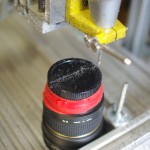
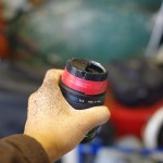
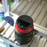
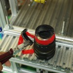
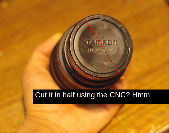
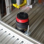
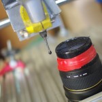
This is an update on my camera lens fail post, where my Tamron rear lens cap got permanently stuck on a Samyang lens. Here is the picture story of how it went down.

Camera lens FAIL

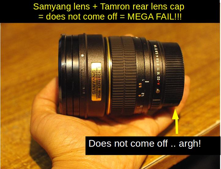
Over the weekend I was shooting with my new Samyang 85mm F1.4 and decided to swap it over with a Sigma 30mm F1.4 to do wider shooting. I had a Tamrom rear lens cap in the bag so I used that. I’m lazy when it comes to camera, I just re-use the same rear lens cap for every lens, one size fit all. Never had an issue until recently. The picture below summarises what happened:

Samyang 85mm F1.4 with Tamron rear lens cap

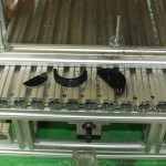
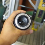
So what now? My initial plan is to use the CNC as shown below.

What could go wrong? Well, we’ll find out soon enough!

Using Maxima to help write compact and fast matrix maths code and more

I’ve recently discovered this cool piece of open source software called Maxima. For those unfamiliar, it is a Computer Algebra System (CAS). You can express maths problem using symbols (as oppose to numerical values only) and apply common maths operations like integration, differentiation, matrix manipulation, finding roots, solving for x, simplificationĀ  etc. etc. to name a few. In fact, it could probably do most of your calculus homework for you, provided the teacher overlooks the fact that you didn’t show any working step.

Maxima operates on the command line but I tend to use the GUI frontend wxMaxima.

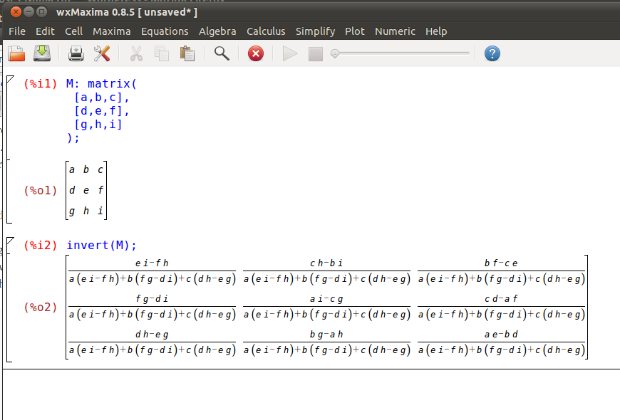
Here’s a programming scenario, you need to do a simple matrix operation, like an inversion of a 3×3 matrix to solve a linear problem. You want it fast but don’t want the hassle of linking to an external library, for whatever reason. Sure, you could do a quick Google and probably find an answer or use it as an excuse to play with Maxima. Here is how to do this in wxMaxima.

3x3 matrix inversion

M is the 3×3 matrix with each element index by some letter. The output can now be translated directly into C, C++ code or whatever your favourite language is. Notice how the denominator is all the same, so you can improve efficiency by storing it into a variable. You can also check if the denominator is near zero, which would indicate a singular matrix that can’t be inverted.

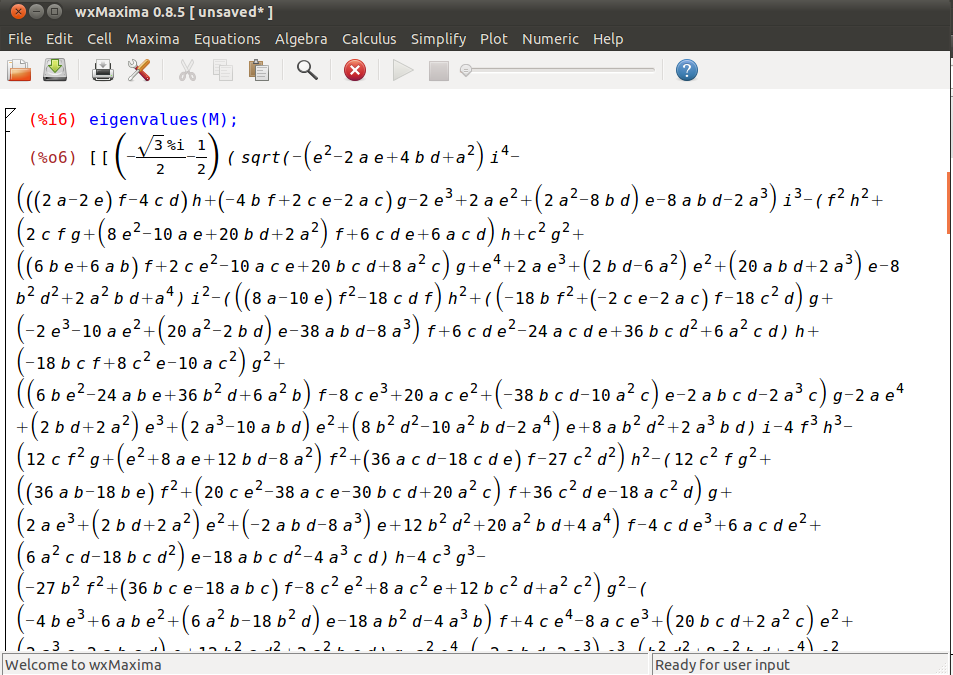
Eigenvalues of a 3×3 matrix? Sure !

Eigenvalues of a 3x3 matrix
Eigenvalues of a 3x3 matrix ... bad idea

Err okay, maybe not such a great idea.

Need to solve Ax = b? Just re-arrange to x = invert(A)b and you got your answers. You probably only need one IF statement and the rest are maths operation. Not a single FOR loop. How’s that for lean and mean code.

Simple Pano Stitcher

In the past I’ve received emails from people on the OpenCV Yahoo group asking for help on panoramic stitching, to which I answered them to the best of my knowledge, though the answers were theoretical. Being the practical man I like to think of myself,  I decided to finally get down and dirty and write a simple panoramic stitcher that should help beginners venturing into panoramic stitching. In the process of doing so I learned some new things along the way. I believe OpenCV is scheduled to include some sort of panoramic stitching engine in future release. In the meantime you can check out my Simple Pano Stitcher program here:

Last update: 31/03/2014

Download SimplePanoStitcher-0.2.0.zip

It uses OpenCV to do fundamental image processing stuff and includes a public domain Levenberg-Marquardt non-linear solver.

To compile the code just type make and run bin/Release/SimplePanoStitcher. It will output a bunch of layer-xxx.png images as output. I’ve included sample images in the sample directory, which the program uses by default. Edit the source code to load your own images. You’ll need to know the focal length in pixels used to capture each image.

To keep things simple I only wrote the bare minimum to get it up and running, for more information check the comments in main.cpp at the top of the file.

Results with Simple Pano Stitcher

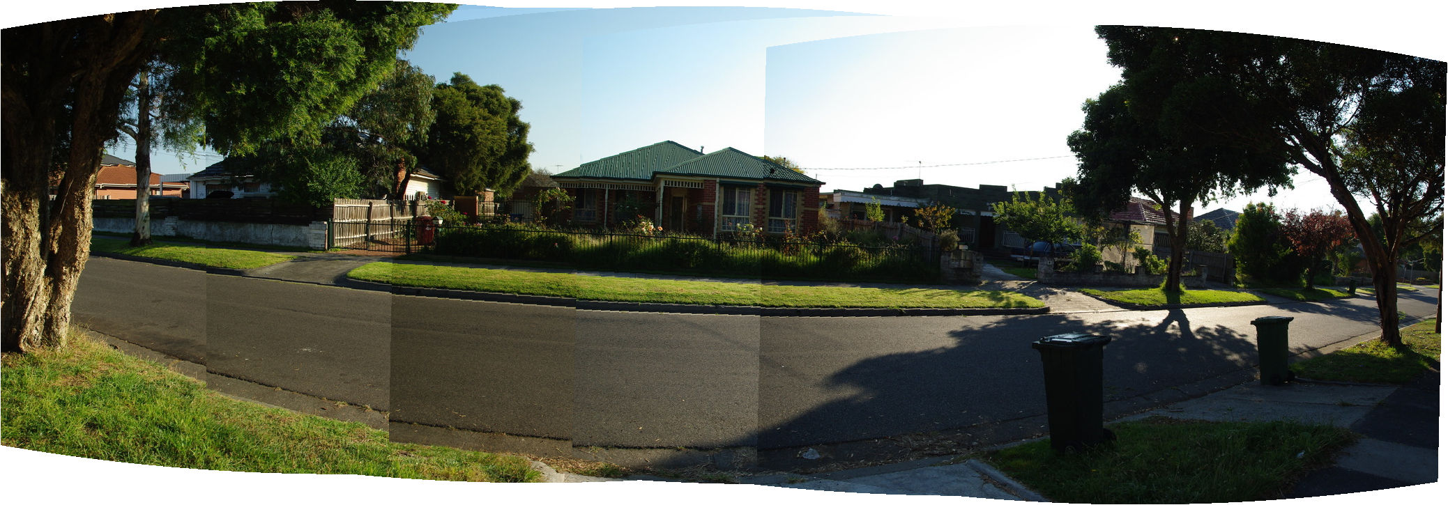
Below is a sample result I got after combining all the layers, by simply pasting them on top of each other. No fancy blending or anything. On close inspection there is some noticeable parallax. If I had taken it on a tripod instead of hand held it should be less noticeable.

Sample results from Simple Pano Stitcher

Discussion

One of the crucial steps to getting good results is the non-linear optimisation step. I decided to optimise the focal length, yaw, pitch, and roll for each image. A total of 4 parameters. I thought it would be interesting to compare results with and without any optimisation. For comparison I’ll be using the full size images (3872 x 2592), which is not included in the sample directory to keep the package size reasonable. Below shows a close up section of the roof of the house without optimisation.

Panoramic stitching without non-linear optimisation

The root mean squared error reported is 22.5008 pixels. The results are without a doubt awful! Looking at it too long would cause me to require new glasses with a stronger optical prescription. I’ll now turn on the non-linear optimisation step for the 4 parameters mentioned previously. Below is what we get.

Panoramic stitching with optimisation
Panoramic stitching with non-linear optimisation

The reported root mean squared error is 3.84413 pixels. Much better! Not perfect, but much more pleasant to look at than the previous image.

There is no doubt a vast improvement by introducing non-linear optimisation to panoramic stitching. One can improve the results further by taking into consideration for radial distortion, but I’ll leave that as an exercise to the reader.

I originally got the focal length for my camera lens from calibration using the sample program (calibration.cpp) in the OpenCV 2.x directory. It performs a standard calibration using a checkerboard pattern. Yet even then its accuracy is still a bit off. This got me thinking a bit. Can we use panoramic stitching to refine the focal length? What are the pros and cons? The images used in the stitching process should ideally be scenery with features that are very very far, so that parallax is not an issue, such as outdoor landscape of mountains or something. Seems obvious enough, there are probably papers out there but I’m too lazy to check at this moment …

OpenCV port of ‘Robust Pose Estimation from a Planar Target’

Please see this page for the most up to date information regarding this post and code.

A few months ago I wrote an OpenCV version of the pose estimation algorithm found in the paper Robust Pose Estimation from a Planar Target (2006) by Gerald Schweighofer and Axel Pinz using their Matlab code from the link in the paper.

I originally ported it so I could play around with Augmented Reality, specifically to track a planar maker (business card). Although that project hasn’t received much attention lately I figured someone might find the pose estimation part useful. IĀ  was about to post it up last night when I came across a small bug, which took 2-3 hour to hunt down. Seems like the new OpenCV Mat class has some subtle gotchas but all good now.I checked my results with the original Matlab code and they appear numerically the same, which is always a good sign.

Download RobustPlanarPose-1.1.2.zip

Look at demo.cpp to see how it works.

UPDATE: 12 March 2012

If you plan to use this for Augmented Reality applications then you should modify Line 23 in RPP.cpp from:

ObjPose(model_3D, iprts, NULL, &Rlu, &tlu, &it1, &obj_err1, &img_err1);

to

ObjPose(model_3D, iprts, &Rlu, &Rlu, &tlu, &it1, &obj_err1, &img_err1);

This initialise the guess of the rotation matrix to the last estimate, providing smoother and more accurate results.

KD-tree on GPU for 3D point searching

This post is a follow up on my previous post about using the GPU for brute force nearest neighbour searching. In the previous post I found the GPU to be slower than using the ANN library, which utilises some sort of KD-tree to speed up searches. So I decided to get around to implementing a basic KD-tree on the GPU for a better comparison.

My approach was to build the tree on the host and transfer it to the GPU.Ā  Sounds conceptually easy enough, as most things do. The tricky part was transferring the tree structure. I ended up representing the tree as an array node on the GPU, with each node referencing other nodes using an integer index, rather than using pointers, which I suspect would have got rather ugly. The KD-tree that I coded allows the user to set the maximum depth if they want to, which turned out to have some interesting effects as shown shortly.Ā  But first lets see some numbers:

nghia@nghia-laptop:~/Projects/CUDA_KDtree$ bin/Release/CUDA_KDtree
CUDA blocks/threads: 196 512
Points in the tree: 100000
Query points: 100000

Results are the same!

GPU max tree depth: 99
GPU create + search: 321.849 + 177.968 = 499.817 ms
ANN create + search: 162.14 + 456.032 = 618.172 ms
Speed up of GPU over CPU for searches: 2.56x

Alright, now we’re seeing better results from the GPU. As you can see I broken the timing down for the create/search part of the KD-tree. My KD-tree creation code is slower than ANN, no real surprise there. However the searches using the GPU is faster, the results I was hoping for. But only 2.56x faster, nothing really to rave about. I could probably get the same speed up, or more, by multi-threading the searches on the CPU. I then started to play around with the maximum depth of my tree and got these results:

GPU max tree depth: 13
GPU create + search: 201.771 + 56.178 = 257.949 ms
ANN create + search: 163.414 + 403.978 = 567.392 ms
Speed up of GPU over CPU for searches: 7.19x

From 2.56x to 7.19x, a bit better! A max tree depth of 13 produced the fastest results. It would seem that there is a sweet spot between creating a tree with the maximum depth required, so that each leaf of the tree holds only a single point, versus a tree with a limited depth and doing a linear search on the leaves. I suspect most of the bottleneck is due to the heavy use of global memory, especially randomly accessing them from different threads, which is why we’re not seeing spectacular speed ups.

The code for the CUDA KD-tree can be downloaded here CUDA_KDtree.zip. Its written for Linux and requires the ANN library to be installed.

Brute Force Nearest Neighbour in CUDA for 3D points

It has been a while since I touched CUDA and seeing as I haven’t posted anything interesting on the front page yet I decided to write a simple brute force nearest neighbour to pass time. The idea has been implemented by the fast kNN library. The library is restricted to non-commerical purposes.

In the past I’ve needed to do nearest neighbour search mainly in 3D space, particular for the Iterative Closest Point (ICP) algorithm, or the likes of it. I relied on the ANN library to do fast nearest neighbour searches, which it does very well. A brute force implementation at the time would have been unimaginably slow and simply impractical. It would have been as slow as watching paint dry for the kind of 3D data I worked on. On second thoughts, watching paint dry would have been faster. Brute force has a typical running time of O(NM), where N and M are the size of the two data set to be compared, basically quadratic running time if both data sets are similar in size. This is generally very slow and impractical for very large data set using the CPU. You would almost be crazy to do so. But on the GPU it is a different story.

I ran a test case where I have 100,000 3D points and 100,000 query points. Each query point searches for its nearest point. This equates to 100,000,000,000 comparisons (that’s a lot of zeros, did I count them right? yep I did). This is what I got on my Intel i7 laptop with a GeForce GTS 360M:

nghia@nghia-laptop:~/Projects/CUDA_NN$ bin/Release/CUDA_NN
Data dimension: 3
Total data points: 100000
Total query points: 100000

GPU: 2193.72 ms
CPU brute force: 69668.3 ms
libANN: 540.008 ms

Speed up over CPU brute force from using GPU: 31.76x
Speed up over libANN using GPU: 0.25x

ANNĀ  produces the fastest results for 3D point searching. The GPU brute force version is slower but still practical for real applications, especially given its ease of implementation and reasonable running time.

I’d imagine even greater speed up (orders of magnitude?) is achievable with a KD-tree created on the GPU. A paper describing building a KD-tree on the GPU can be found at http://www.kunzhou.net/.Ā  However I could not find any source code on the website. I might give it a shot when I have time.

The demo code I wrote only searches for the nearest point given a query point. Extending the program to find the K nearest neighbour for a bunch of query points should not be too difficult. Each query point would have to maintain a sorted array of indexes and distances.

My code can be downloaded here (CUDA_LK.zip). If you’re on Linux just type make and run CUDA_NN. Just a warning, on Linux if a CUDA program runs for more than 5 second or so the operating system will kill it and display some warning.