Last Updated on April 4, 2017 by nghiaho12
With some more free time lately I’ve decided to get back into some structure from motion (SFM). In this post I show a simple SFM pipeline using a mix of OpenCV, GTSAM and PMVS to create accurate and dense 3D point clouds.
This code only serves as an example. There is minimal error checking and will probably bomb out on large datasets!
Code
https://github.com/nghiaho12/SFM_example
You will need to edit src/main.cpp to point to your dataset or you test with my desk dataset.
http://nghiaho.com/uploads/desk.zip
Introduction
There are four main steps in the SFM pipeline code that I will briefly cover
If your code editor supports code folding you can turn it on and see each step locally scoped around curly braces in src/main.cpp.
To simplify the code I assume the images are taken sequentially, that is each subsequent image is physically close and from the same camera with fixed zoom.
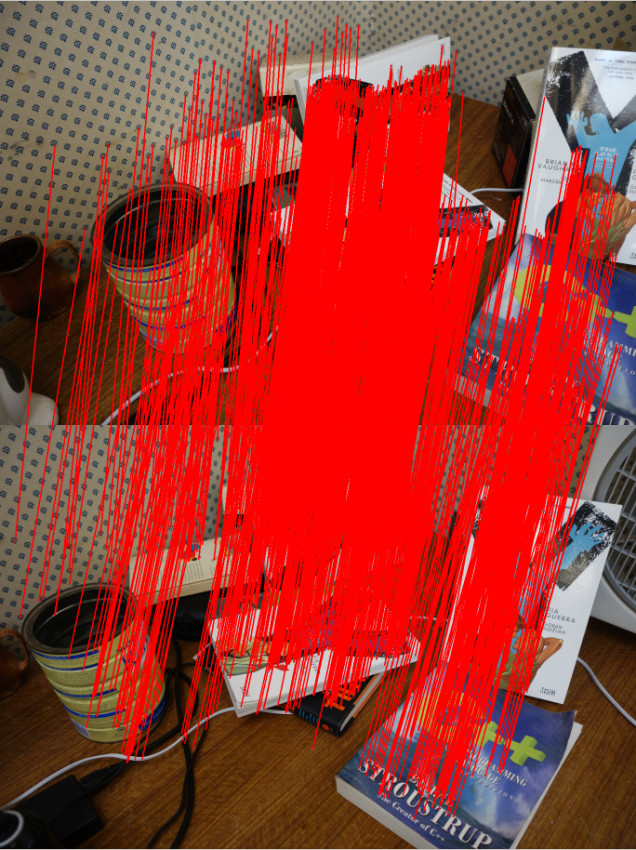
Feature matching
The first step is to find matching features between the images. There are many OpenCV tutorial on feature matching out there so I won’t go into too much detail.
There are a few ways to go about picking pair of images to match. In my code I match every image to each other. So if there N images, there are N*(N-1)/2 image pairs to match. This of course can get pretty slow since it scales quadratically with the number of images.
I initially tried ORB but found AKAZE to produce more matches. Matches have to past a ratio test (best match vs second best match) and the fundamental matrix constraint to be kept.
The only slightly tedious part is the book keeping of matched features. You need to keep track of features that match across many images. For example, a feature in image 0 may have a match in image 1 and image2. This is important because features that are seen in at least 3 views allow us to recover relative scale between motion.
Motion recovery and triangulation
This is the core part of the SFM pipeline and I take advantage of the following OpenCV functions
- cv::findEssentialMat
- cv::recoverPose
- cv::triangulatePoints
cv::findEssentialMat uses the 5-point algorithm to calculate the essential matrix from the matched features. It’s the de-facto algorithm for finding the essential matrix and is superior to the 8-point algorithm when used in conjunction with RANSAC to filter out outliers. But it is not easy to code up from scratch compared to the 8-point.
The pose from the essential matrix is recovered by cv::recoverPose. It returns a 3×3 rotation (R) and translation vector (t). The pose at camera n is calculated as follows
![T_n = T_{n-1}\left[\begin{array}{ccc|c} & & \\ & R & & t\\ & & \\ 0 & 0 & 0 & 1 \end{array}\right]](https://s0.wp.com/latex.php?latex=T_n+%3D+T_%7Bn-1%7D%5Cleft%5B%5Cbegin%7Barray%7D%7Bccc%7Cc%7D+%26+%26+%5C%5C+%26+R+%26+%26+t%5C%5C+%26+%26+%5C%5C+0+%26+0+%26+0+%26+1+%5Cend%7Barray%7D%5Cright%5D&bg=ffffff&fg=000000&s=0 "T_n = T_{n-1}\left[\begin{array}{ccc|c} & & \\ & R & & t\\ & & \\ 0 & 0 & 0 & 1 \end{array}\right]")
 is a 4×4 matrix.
Given two poses the 2D image points can then be triangulated using cv::triangulatePoints. This function expects two projection matrices (3×4) as input. To make a projection matrix from the pose you also need the camera matrix K (3×3). Let’s say we break up the pose matrix 

![T_n = \left[\begin{array}{ccc|c} & & \\ & R_n & & t_n\\ & & \\ 0 & 0 & 0 & 1 \end{array}\right]](https://s0.wp.com/latex.php?latex=T_n+%3D+%5Cleft%5B%5Cbegin%7Barray%7D%7Bccc%7Cc%7D+%26+%26+%5C%5C+%26+R_n+%26+%26+t_n%5C%5C+%26+%26+%5C%5C+0+%26+0+%26+0+%26+1+%5Cend%7Barray%7D%5Cright%5D&bg=ffffff&fg=000000&s=0 "T_n = \left[\begin{array}{ccc|c} & & \\ & R_n & & t_n\\ & & \\ 0 & 0 & 0 & 1 \end{array}\right]")
The 3×4 projection matrix for the camera n is
![P_n = K\left[\begin{array}{c|c} R_n^T & -R_n^{T}t_n\end{array}\right]](https://s0.wp.com/latex.php?latex=P_n+%3D+K%5Cleft%5B%5Cbegin%7Barray%7D%7Bc%7Cc%7D+R_n%5ET+%26+-R_n%5E%7BT%7Dt_n%5Cend%7Barray%7D%5Cright%5D&bg=ffffff&fg=000000&s=0 "P_n = K\left[\begin{array}{c|c} R_n^T & -R_n^{T}t_n\end{array}\right]")
This process is performed sequentially eg. image 0 to image 1, image 1 to image 2.
There is an ambiguity in the scale recovered from the essential matrix (hence only 5 degrees of freedom). We don’t know the length of the translation between each image, just the direction. But that’s okay, we can use the first image pair (image 0 and image 1) and use that as the reference for relative scale. An illustration of how this is done is shown below. Click on the image to zoom in.
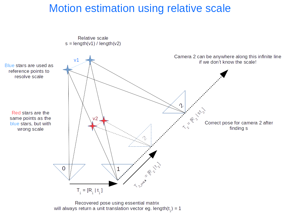
The following calculations occurs
- Recover motion between image 0 and 1 and triangulate to get the blue points. These points will be used as the reference to figure out the relative scale.
- Recover motion between image 1 and image 2 and triangulate to get the red points. Using our 2D feature matching done earlier we find that they are the same as the blue points. The rotation (
) is correct, but the translation (
) needs to be scaled.
- Find the relative scale by picking a pair of blue points and the matching red points and calculate the ratio of the vector lengths.
- Apply the scale to
Everything I’ve outlined so far is the basically visual odometry. This method only works if the images are taken sequentially apart.
Bundle adjustment
Everything we’ve done so far more or less works but is not optimal, in the statistical sense. We have not taken advantage of constraints imposed by features matched across multiple views nor have we considered uncertainty in the measurement (the statistical part). As a result, the poses and 3D points recovered won’t be as accurate as they can be. That’s where bundle adjustment comes in. It treats the problem as one big non-linear optimization. The variables to be optimized can include all the poses, all the 3D points and the camera matrix. This isn’t trivial to code up from scratch but fortunately there are a handful of libraries out there designed for this task. I chose GTSAM because I was learning it for another application. They had an example of using GTSAM for SFM in the example directory, which I based my code off.
Output for PMVS
After performing bundle adjustment we have a good estimate of the poses and 3D points. However the point cloud generally isn’t dense. To get a denser point cloud we can use PMVS. PMVS only requires the 3×4 projection matrix for each image as input. It will generate its own features for triangulation. The projection matrix can be derived from the poses optimized by GTSAM.
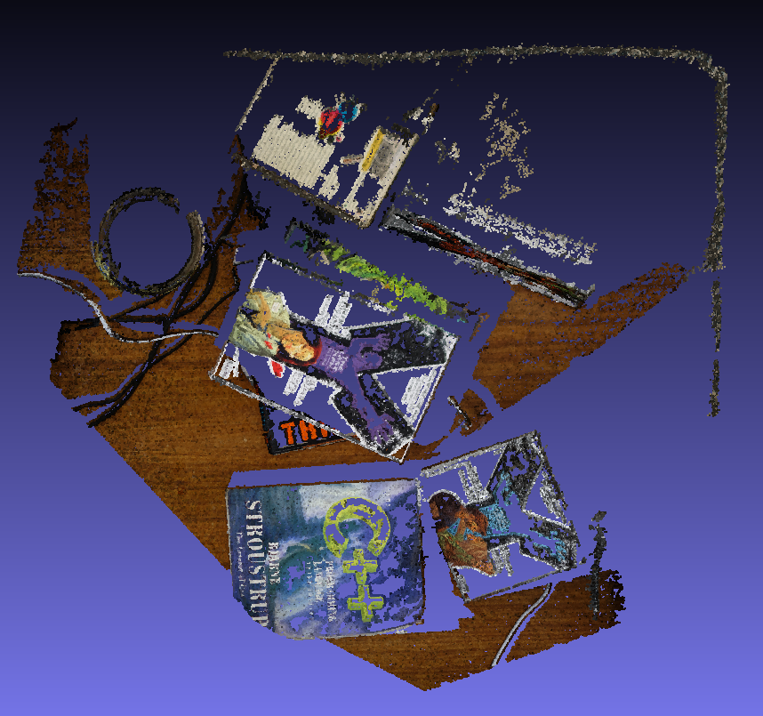
Example
Here’s a dataset of my desk you can use to verify everything is working correctly.
http://nghiaho.com/uploads/desk.zip
Here’s a screenshot of the output point cloud in Meshlab.
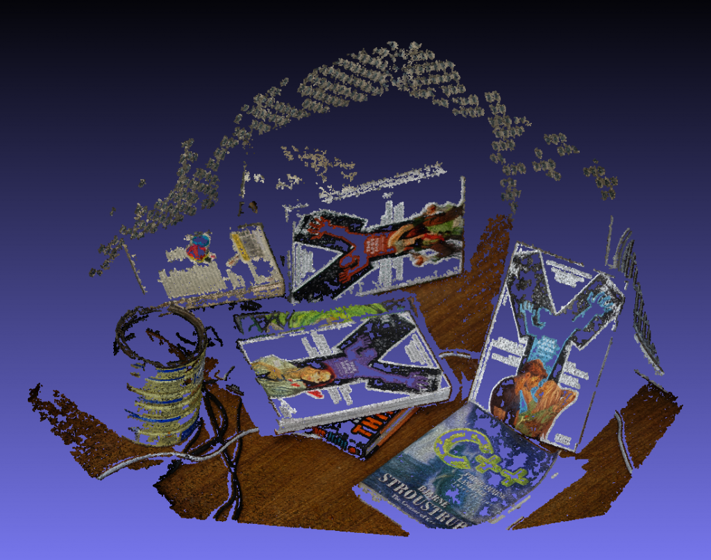
If you set Meshlab to display in orthographic mode you can see the walls make a right angle.
References
http://rpg.ifi.uzh.ch/visual_odometry_tutorial.html