Category Archives: Technical
A bunch of technical posts to help me remember useful stuff, should I become senile in the future.
CIFAR10 with fastai
Numpy images with fastai
Using the iPhone TrueDepth Camera as a 3D scanner
A friend of mine from PunkOffice (punkoffice.com) recently hit me up and asked if I knew how to register a bunch of point clouds from his shiny Apply iPhone 11 that comes with a TrueDepth camera. He was interested in using it as a portable 3D scanner. Why yes I do! At least I did over a decade ago for my PhD. Back then I used the popular ICP (Iterative Closest Point) algorithm to do point-to-point registration. It did the job. But I wasn’t in the mood to reinvent the wheel again. So instead I searched for existing Python libraries that would get the job done with the least amount of effort. In my search I came across the Open3D library (http://open3d.org) that comes with Python bindings. This library includes file loaders for various 3D formats, a handful of registration methods, and a visualizer. Perfect!
What was meant to be a quick proof of concept eventually evolved into a mini R&D project as I sought for better registration accuracy!
The code is at the bottom of the page.
Problem we’re trying to solve
Essentially we’re trying to solve for the camera poses, that is its orientation and translation in 3D space. If we know the camera poses then creating a 3D point cloud from the individual captures is easy, we just project the 3D point out at that pose and we’re done. To do this we need to know the TruthDepth camera’s calibration and a dataset to work with.
Apple TrueDepth camera calibration
The first step was to gather any useful information about the TruthDepth camera. Apple has an API that allows you to query calibrationn data of the camera. I told my friend what I was looking for and he came back with the following
- raw 640×480 depth maps (16bit float)
- raw 640x480x3 RGB images (8bit)
- camera intrinsics for 12MP camera
- lens distortion lookup (vector of 42 floats)
- inverse lens distortion lookup (vector of 42 floats)
Some intrinsic values
- image width: 4032
- image height: 3024
- fx: 2739.79 (focal)
- fy: 2739.79 (focal)
- cx: 2029.73 (center x)
- cy: 1512.20 (center y)
This is fantastic, because it means I don’t have to do a checkerboard calibration to learn the intrinsics. Everything we need is provided by the API. Sweet!
The camera intrinsics is for a 12MP image, but we’re given a 640×480 image. So what do we do? The 640×480 is simply a scaled version of the 12MP image, meaning we can scale down the intrinsics as well. The 12MP image aspect ratio is 4032/3204 = 1.3333, which is identical to 640/480 = 1.3333. The scaling factor is 640/4032 = 0.15873. So we can scale [fx, fy, cx, cy] by this value. This gives the effective intrinisc as
- image width: 640
- image height: 480
- fx: 434.89
- fy: 434.89
- cx: 322.18
- cy: 240.03
Now the distortion is interesting. This is not the usual radial distortion polynomial paramterization. Instead it’s a lookup table to determine how much scaling to apply to the radius. This is the first time I’ve come across this kind of expression for distortion. A plot of the distortion lookup is shown below

Here’s some pseudo code to convert an undistorted point to distorted point
def undistort_to_distort(x, y):
  xp = x - cx
  yp = y - cy
  radius = sqrt(xp*xp + yp*yp)
  normalized_radius = radius / max_radius

  idx = normalized_radius*len(inv_lens_distortion_lookup)
  scale = 1 + interpolate(inv_lens_distortion_lookup, idx)

  x_distorted = xp*scale + cx
  y_distorted = yp*scale + cy

  return x_distorted, y_distorted
idx will be a float and you should interpolate for the correct value, rather than round to the nearest integer. I used linear interpolation. To go from distorted to undistorted switch inv_lens_distortion_lookup with lens_distortion_lookup.
With a calibrated camera, we can project a 2D point to 3D as follows.
def project_to_3d(x, y, depth):
  xp = (x - xc)/fx * depth
  yp = (y - yc)/fy * depth
  zp = depth

  return [xp, yp, zp]
I found these links helpful when writing up this section.
- https://frost-lee.github.io/rgbd-iphone/
- https://developer.apple.com/documentation/avfoundation/avcameracalibrationdata
Dataset
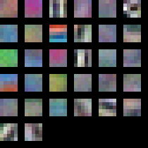
The dataset I got from my friend consists of 40 captures, which includes both RGB images and depth maps as shown below. I’m showing a gray image to save file space and I segmented the depth map to isolate the objects so you can see it better. There’s a box with a tin can on top, which are two simple shapes that will make it easy to compare results later on. The camera does a 360 or so degree pan around the object, which we’ll exploit later on as well.


Method #1 – Sequential ICP
The simplest method I could think of is sequential ICP. In this method the current point cloud is registered to the previous. I used Open3D’s point-to-plane variant of ICP, which claims better performance than point-to-point ICP. ICP requires you to provide an initial guess of the transform between the point clouds. Since I don’t have any extra information I used the identity matrix, basically assuming no movement between the captures, which of course isn’t true but it’s a good enough guess.
Below shows a top down view of the box and can. You can some misalignment of the box on the right side. This will be our baseline.

Method #2 – Sequential vision based
There are two drawbacks with the sequential ICP approach. First, using 3D points alone can not resolve geometric ambiguities. For example, if we were to capture a sequence of a flat wall, ICP would struggle to find the correct transform. Second, ICP needs an initial transform to boot strap the process.
To address these shortcomings ‘ll be using both the image and depth data. The image data is richer for tracking visual features. Here is an outline the approach
1. Track 2D SIFT features from current to previous frame
2. Use the fundmanmetal matrix to filter out bad matches
3. Project the remaining 2D points to 3D
4. Find the rigid transform between current and previous 3D points
We now have a good estimate for the transform between camera poses, rather than assume identity transform like with ICP!
The advantage estimating the transform in 3D is it’s much easier and possibly than traditional 2D approaches. The rigid transform can be calculated using a closed form solution. The traditional 2D approach requires calculating the essential matrix, estimating 3D points, solving PnP, … And for a monocular camera it’s even trickier!
Here’s the result of the sequential vision based approach

Hmm no noticeable improvement. Sad face. Still the same problem. Fundamentally, our simplistic approach of registering current to previous introduces a small amount of drift over each capture.
Oh fun fact, the SIFT patent expired some time early 2020! It got moved out of OpenCV’s non-free module and is now back in the features2d module.
Method #3 – Sequential vision based with loop closure detection
To reduce the effect of drift and improve registration we can exploit the knowledge that the last capture’s pose is similar to one of the earlier capture, as the camera loops back around the object. Once we find the loop closure match and the transform between them we can formulate this as a pose graph, plus feature matching constraints, and apply an optimization. Pose graph optimization is commonly used in the robotics community to solve for SLAM (simultaneous localization and mapping) type of problems. There are 3 main ingredients for this optimization
1. define the parameters to be optimized
2. define the cost function (constraint)
3. provide good initial estimates of the parameters
As mentioned earlier, we’re interested in solving for the camera poses (rotation, translation). These are the parameters we’re optimizing for. I chose to represent rotation as a Quaternion (4D vector) and translation as a 3D vector (xyz). So a total of 7 parameters for each camera. It’s also common to represent the rotation using an axis-angle parameterization, such that it’s a 3D vector. This will be faster to optimize but there are singularities you have to watch out for. See http://www.euclideanspace.com/maths/geometry/rotations/conversions/matrixToAngle for more insight. The Quaternion doesn’t have this problem, but requires the solver to make sure the vector is unit length to be a valid rotation vector.
For the cost function, given the current parameters, I want to minimize the Euclidean distance between the matching 3D points. Here’s a pseudo code for the cost function
def cost_func(rot1, trans1, rot2, trans2, pts1, pts2):
  # rot1, rot2 - quaternion
  # trans1, trans2 - 3D translation
  # pts1, pts2 - matching 3D point

  pts1_ = rotate_point(rot1, pts1) + trans1
  pts2_ = rotate_point(rot2, pts2) + trans2

  residuals[0] = pts1_.x - pts2_.x
  residuals[1] = pts1_.y - pts2_.y
  residuals[2] = pts1_.z - pts2_.z

  return residuals
We add a cost function for every 3D match. So this includes all the current to previous matches plus the loop closure match. The optimization algorithm will adjust the parameters iteratively to try and make the loss function approach zero. A typical loss function is loss = sum(residuals^2), this is the familiar least squares.
Pose graph optimization uses a non-linear optimization method, which requires the user to provide a good estimate of the parameters else it will converge to the wrong solution. We will use approach #2 to initialize our guess for the camera poses.
I used Ceres Solver to solve the pose graph. The results are shown below.
All the box edges line up, yay!
Method #4 – Sequential ICP with loop closure detection
Let’s revisit sequential ICP and see if we can add some pose graph optimization on top. Turns out Open3D has a built in pose graph optimizer with some sample code! Here’s what we get.

Better then vanilla sequential ICP, but not quite as good as the vision based method. Might just be my choice in parameters.
More improvements?
We’ve seen how adding loop closure to the optimization made a significant improvement in the registration accuracy. We can take this idea further and perform ALL possible matches between the captures. This can get pretty expensive as it scales quadratically with the number of images, but do-able. In theory, this should improve the registration further. But in practice you have to be very careful. The more cost functions/constraints we add the higher the chance of introducing an outlier (bad matches) into the optimization. Outliers are not handled by the simple least square loss function and can mess things up! One way to handle outliers is to use a different loss function that is more robust (eg. Huber or Tukey).
You can take the optimization further and optimize for the tracked 3D points and camera intrinsics as well. This is basically bundle adjustment found in the structure from motion and photogrammetry literature. But even with perfect pose your point cloud is still limited by the accuracy of the depth map.
Summary of matching strategies
Here’s a graphical summary of the matching strategies mentioned so far. The camera poses are represented by the blue triangles and the object of interest is represented by the cube. The lines connecting the camera poses represents a valid match.
Sequential matching
Fast and simple but prone to drift the longer the sequence. Matching from capture to capture is pretty reliable if the motion is small between them. The vision based should be more reliable than ICP in practise as it doesn’t suffer from geometric ambiguities. The downside is the object needs to be fairly textured.

Vision based sequential matching with loop closure detection
An extension of sequential matching by explicitly detecting where the last capture loops back with an earlier capture. Effectively eliminates drift. It involves setting up a non-linear optimization problem. This can be expensive if you have a lot of parameters to optimize (lots of matched features). The loop closure detection strategy can be simple if you know how your data is collected. Just test the last capture with a handful of the earlier capture (like 10), and see which one has the most features matched. If your loop closure detection is incorrect (wrong matching pair of capture) then the optimization will fail to converge to the correct solution.

Finding all matches
This is a brute force method that works even if the captures are not ordered in any particular way. It’s the most expensive to perform out of the three matching strategies but can potentially produce the best result. Care must be taken to eliminate outliers. Although this applies to all method, it is more so here because there’s a greater chance of introducing them into the optimization.

Alternative approaches from Open3D
Open3D has a color based ICP algorithm (http://www.open3d.org/docs/release/tutorial/Advanced/colored_pointcloud_registration.html) that I have yet to try out but looks interesting.
There’s also a 3D feature based registration method that doesn’t require an initial transform for ICP but I haven’t had much luck with it.
http://www.open3d.org/docs/release/tutorial/Advanced/global_registration.html
Meshing
Open3D also includes some meshing functions that make it easy to turn the raw point cloud to a triangulated mesh. Here’s an example using Poisson surface reconstruction. I also filter out noise by only keeping the largest mesh, that being the box and tin can. Here it is below. It even interpolated the hollow top of the tin can. This isn’t how it is in real life but it looks kinda cool!

Final thoughts
Depending on your need and requirement you should always advantage of any knowledge of how the data was collected. I’ve shown a simple scenario where the user pans around an object. This allows for some simple and robust heuristics to be implemented. But if your aiming for something more generic, where there’s little restriction on the data collecting process, then you’re going to have to write more code to handle all these cases and make sure they’re robust.
Code
OpenCV camera in Opengl
In this post I will show how to incorporate OpenCV’s camera calibration results into OpenGL for a simple augmented reality application like below. This post will assume you have some familiarity with calibrating a camera and basic knowledge of modern OpenGL.

Background
A typical OpenCV camera calibration will calibrate for the camera’s intrinsics
- focal length (fx, fy)
- center (cx, sy)
- skew (usually 0)
- distortion (number of parameters depends on distortion model)
In addition it will also return the checkerboard poses (rotation, translation), relative to the camera. With the first 3 intrinsics quantities we can create a camera matrix that projects a homogeneous 3D point to 2D image point
\[camera \times X = \begin{bmatrix}
f_x & s & c_x & 0 \\
0 & f_y & c_y & 0 \\
0 & 0 & 1 & 0 \\
0 & 0 & 0 & 1
\end{bmatrix}
\times
\begin{bmatrix}
x \\ y \\ z \\ 1
\end{bmatrix}
=
\begin{bmatrix}
x’ \\ y’ \\ z’ \\ 1
\end{bmatrix}
\]
The 2D homogenous image point can be obtained by dividing x’ and y’ by z (depth) as follows [x’/z’, y’/z’, z’, 1]. We leave z’ untouched to preserve depth information, which is important for rendering.
The checkerboard pose can be expressed as a matrix, where r is the rotation and t is the translation
\[
model =
\begin{bmatrix}
r0 & r1 & r2 & tx \\
r3 & r4 & r5 & ty \\
r6 & r7 & r8 & tz \\
0 & 0 & 0 & 1
\end{bmatrix}
\]
Combining the camera and model matrix we get a general way of projecting 3D points back to 2D. Here X can be a matrix of points.
\[ X’ = camera \times model \times X \]
The conversion to 2D image point is the same as before, divide all the x’ and y’ by their respective z’. The last step is to multiply by an OpenGL orthographic projection matrix, which maps 2D image points to normalized device coordinates (NDC). Basically, it’s a left-handed co-ordinate viewing cube that is normalized to [-1, 1] in x, y, z. I won’t go into the details regarding this matrix, but if you’re curious see http://www.songho.ca/opengl/gl_projectionmatrix.html . To generate this matrix you can use glm::ortho from the GLM library or roll out your own using this definition based on gluOrtho.
Putting it all together, here’s a simple vertex shader to demonstrate what we’ve done so far
#version 330 core
layout(location = 0) in vec3 vertexPosition;

uniform mat4 projection;
uniform mat4 camera;
uniform mat4 model;

void main()
{
    // Project to 2D
    vec4 v = camera * model * vec4(vertexPosition, 1);

    // NOTE: v.z is left untouched to maintain depth information!
    v.xy /= v.z;

    // Project to NDC
    gl_Position = projection * v;
}
When you project your 3D model onto the 2D image using this method it assumes the image has already been undistorted. So you can use OpenCV’s cv::undistort function to do this before loading the texture. Or write a shader to undistort the images, I have not look into this.
Code
https://github.com/nghiaho12/OpenCV_camera_in_OpenGL
If you have any questions leave a comment.
SFM with OpenCV + GTSAM + PMVS
With some more free time lately I’ve decided to get back into some structure from motion (SFM). In this post I show a simple SFM pipeline using a mix of OpenCV, GTSAM and PMVS to create accurate and dense 3D point clouds.
This code only serves as an example. There is minimal error checking and will probably bomb out on large datasets!
Code
https://github.com/nghiaho12/SFM_example
You will need to edit src/main.cpp to point to your dataset or you test with my desk dataset.
https://nghiaho.com/uploads/desk.zip
Introduction
There are four main steps in the SFM pipeline code that I will briefly cover
If your code editor supports code folding you can turn it on and see each step locally scoped around curly braces in src/main.cpp.
To simplify the code I assume the images are taken sequentially, that is each subsequent image is physically close and from the same camera with fixed zoom.
Feature matching
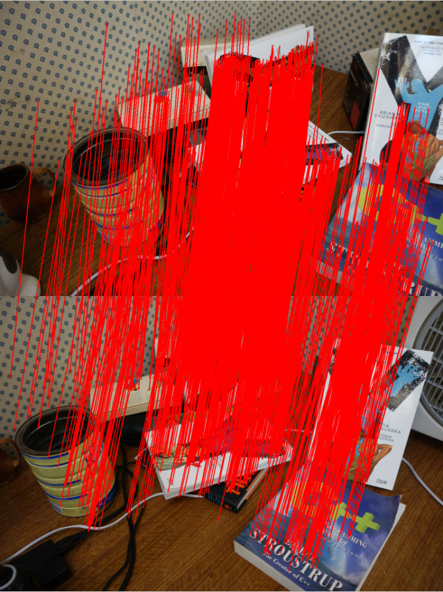
The first step is to find matching features between the images. There are many OpenCV tutorial on feature matching out there so I won’t go into too much detail.
There are a few ways to go about picking pair of images to match. In my code I match every image to each other. So if there N images, there are N*(N-1)/2 image pairs to match. This of course can get pretty slow since it scales quadratically with the number of images.
I initially tried ORB but found AKAZE to produce more matches. Matches have to past a ratio test (best match vs second best match) and the fundamental matrix constraint to be kept.
The only slightly tedious part is the book keeping of matched features. You need to keep track of features that match across many images. For example, a feature in image 0 may have a match in image 1 and image2. This is important because features that are seen in at least 3 views allow us to recover relative scale between motion.
Motion recovery and triangulation
This is the core part of the SFM pipeline and I take advantage of the following OpenCV functions
- cv::findEssentialMat
- cv::recoverPose
- cv::triangulatePoints
cv::findEssentialMat uses the 5-point algorithm to calculate the essential matrix from the matched features. It’s the de-facto algorithm for finding the essential matrix and is superior to the 8-point algorithm when used in conjunction with RANSAC to filter out outliers. But it is not easy to code up from scratch compared to the 8-point.
The pose from the essential matrix is recovered by cv::recoverPose. It returns a 3×3 rotation (R) and translation vector (t). The pose at camera n is calculated as follows
![T_n = T_{n-1}\left[\begin{array}{ccc|c} & & \\ & R & & t\\ & & \\ 0 & 0 & 0 & 1 \end{array}\right]](https://s0.wp.com/latex.php?latex=T_n+%3D+T_%7Bn-1%7D%5Cleft%5B%5Cbegin%7Barray%7D%7Bccc%7Cc%7D+%26+%26+%5C%5C+%26+R+%26+%26+t%5C%5C+%26+%26+%5C%5C+0+%26+0+%26+0+%26+1+%5Cend%7Barray%7D%5Cright%5D&bg=ffffff&fg=000000&s=0 "T_n = T_{n-1}\left[\begin{array}{ccc|c} & & \\ & R & & t\\ & & \\ 0 & 0 & 0 & 1 \end{array}\right]")
 is a 4×4 matrix.
Given two poses the 2D image points can then be triangulated using cv::triangulatePoints. This function expects two projection matrices (3×4) as input. To make a projection matrix from the pose you also need the camera matrix K (3×3). Let’s say we break up the pose matrix 

![T_n = \left[\begin{array}{ccc|c} & & \\ & R_n & & t_n\\ & & \\ 0 & 0 & 0 & 1 \end{array}\right]](https://s0.wp.com/latex.php?latex=T_n+%3D+%5Cleft%5B%5Cbegin%7Barray%7D%7Bccc%7Cc%7D+%26+%26+%5C%5C+%26+R_n+%26+%26+t_n%5C%5C+%26+%26+%5C%5C+0+%26+0+%26+0+%26+1+%5Cend%7Barray%7D%5Cright%5D&bg=ffffff&fg=000000&s=0 "T_n = \left[\begin{array}{ccc|c} & & \\ & R_n & & t_n\\ & & \\ 0 & 0 & 0 & 1 \end{array}\right]")
The 3×4 projection matrix for the camera n is
![P_n = K\left[\begin{array}{c|c} R_n^T & -R_n^{T}t_n\end{array}\right]](https://s0.wp.com/latex.php?latex=P_n+%3D+K%5Cleft%5B%5Cbegin%7Barray%7D%7Bc%7Cc%7D+R_n%5ET+%26+-R_n%5E%7BT%7Dt_n%5Cend%7Barray%7D%5Cright%5D&bg=ffffff&fg=000000&s=0 "P_n = K\left[\begin{array}{c|c} R_n^T & -R_n^{T}t_n\end{array}\right]")
This process is performed sequentially eg. image 0 to image 1, image 1 to image 2.
There is an ambiguity in the scale recovered from the essential matrix (hence only 5 degrees of freedom). We don’t know the length of the translation between each image, just the direction. But that’s okay, we can use the first image pair (image 0 and image 1) and use that as the reference for relative scale. An illustration of how this is done is shown below. Click on the image to zoom in.
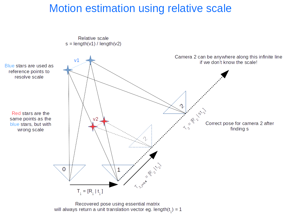
The following calculations occurs
- Recover motion between image 0 and 1 and triangulate to get the blue points. These points will be used as the reference to figure out the relative scale.
- Recover motion between image 1 and image 2 and triangulate to get the red points. Using our 2D feature matching done earlier we find that they are the same as the blue points. The rotation (
) is correct, but the translation (
) needs to be scaled.
- Find the relative scale by picking a pair of blue points and the matching red points and calculate the ratio of the vector lengths.
- Apply the scale to
Everything I’ve outlined so far is the basically visual odometry. This method only works if the images are taken sequentially apart.
Bundle adjustment
Everything we’ve done so far more or less works but is not optimal, in the statistical sense. We have not taken advantage of constraints imposed by features matched across multiple views nor have we considered uncertainty in the measurement (the statistical part). As a result, the poses and 3D points recovered won’t be as accurate as they can be. That’s where bundle adjustment comes in. It treats the problem as one big non-linear optimization. The variables to be optimized can include all the poses, all the 3D points and the camera matrix. This isn’t trivial to code up from scratch but fortunately there are a handful of libraries out there designed for this task. I chose GTSAM because I was learning it for another application. They had an example of using GTSAM for SFM in the example directory, which I based my code off.
Output for PMVS
After performing bundle adjustment we have a good estimate of the poses and 3D points. However the point cloud generally isn’t dense. To get a denser point cloud we can use PMVS. PMVS only requires the 3×4 projection matrix for each image as input. It will generate its own features for triangulation. The projection matrix can be derived from the poses optimized by GTSAM.
Example
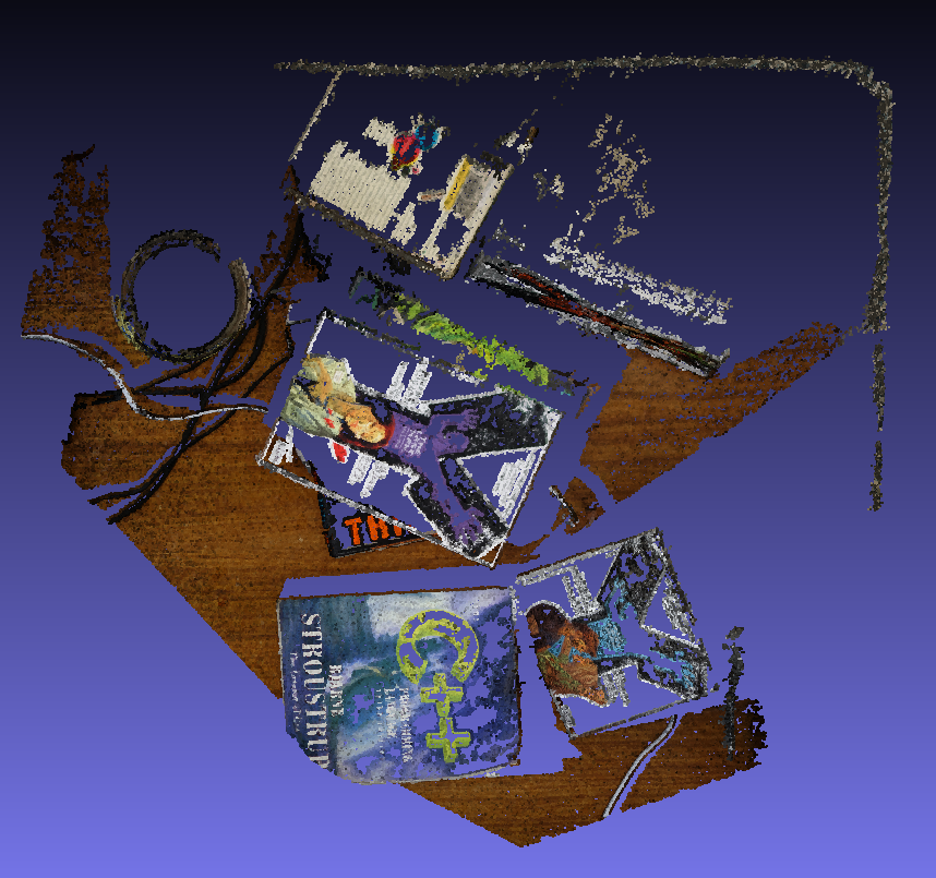
Here’s a dataset of my desk you can use to verify everything is working correctly.
https://nghiaho.com/uploads/desk.zip
Here’s a screenshot of the output point cloud in Meshlab.
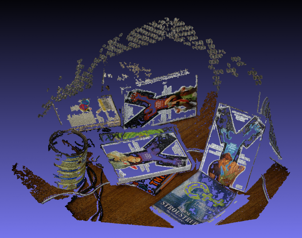
If you set Meshlab to display in orthographic mode you can see the walls make a right angle.
References
http://rpg.ifi.uzh.ch/visual_odometry_tutorial.html
EKF SLAM with known data association
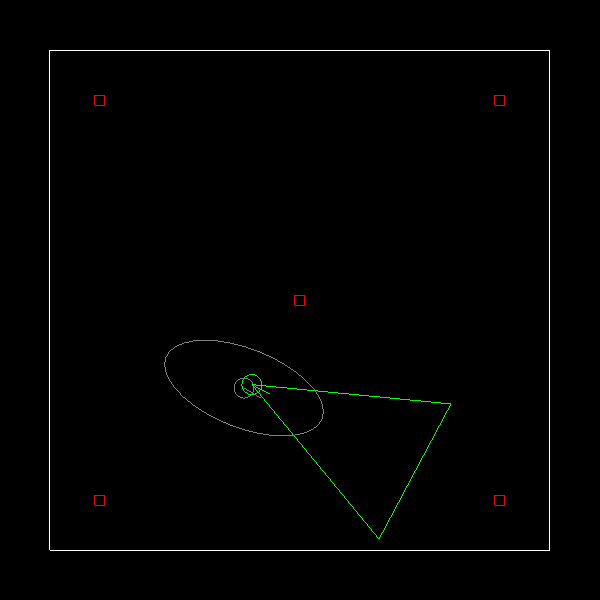
In the previous post I wrote a C++ implementation of the EKF localization algorithm from the Probabilistic Robotics book. As a continuation I also wrote an implementation for the EKF SLAM with known data association algorithm. This is similar to EKF localization except we’re also estimating the landmarks position and uncertainty. The code can be found here.
https://github.com/nghiaho12/EKF_SLAM
Here’s a screenshot of it in action.
EKF localization with known correspondences
Been a while since I posted anything. I recently found some free time and decided to dust off the Probabilistic Robotics book by Thrun et. al. There are a lot of topics in the book that I didn’t learn formally back during school.
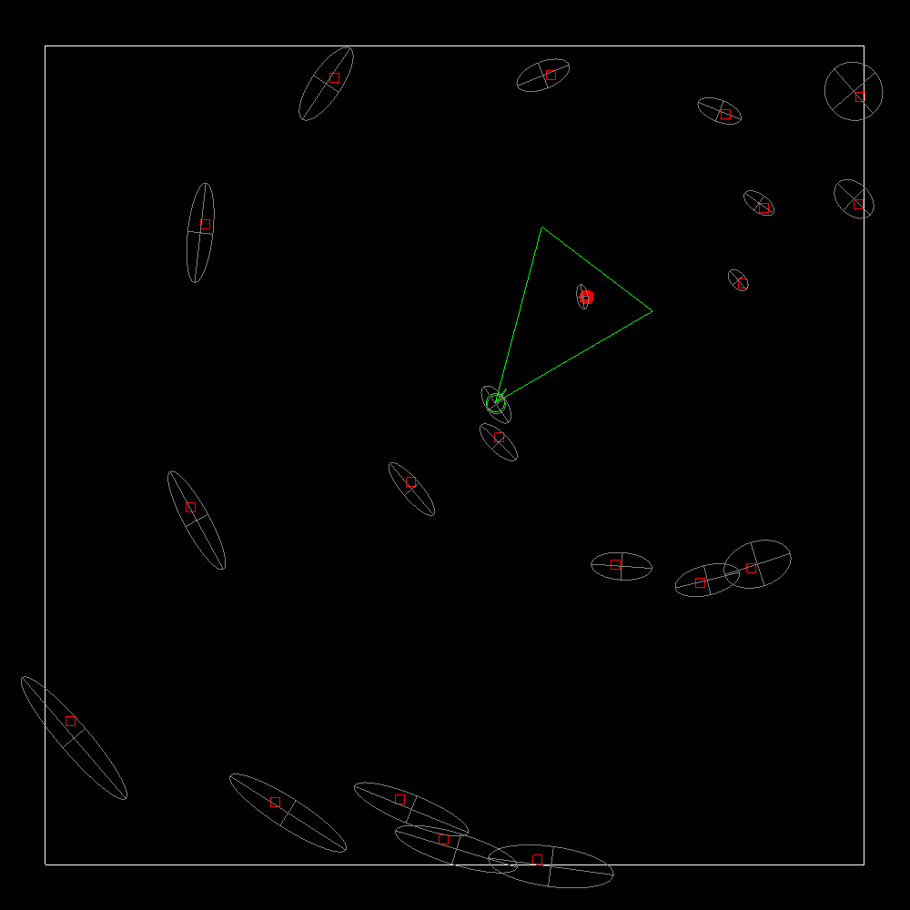
I’ve used the vanilla Kalman Filter for a few projects in the past but not the extended Kalman Filter. I decided to implement the Extended Kalman Filter localization with known correspondences algorithm. The simulation consists of a robot with a range sensor that can detect known landmarks in the world. You move the robot around using the arrow keys. The simulation is written in C++ and uses SDL and OpenGL. Below shows a screenshot. The true pose is in green, gray the EKF estimate and 95% confidence ellipse, red are the landmarks.
One addition I made was handle the case when angular velocity is zero. The original algorithm presented in the book would result in a divide by zero. You can grab and play with the code here.
An interesting behavior that I’ve been trying to understand is the EKF covariance can shrink (reduce uncertainty), even if you are only doing predictions (no correction using landmark). It’s either a coding bug or some side effect of linearization. Either way, it’s driving me nuts!
https://github.com/nghiaho12/EKF_localization_known_correspondences
Using TensorFlow/Keras with CSV files
I’ve recently started learning TensorFlow in the hope of speeding up my existing machine learning tasks by taking advantage of the GPU. At first glance the documentation looks decent but the more I read the more I found myself scratching my head on how to do even the most basic task. All I wanted to do was load in a CSV file and run it through a simple neural network. When I was downloading the necessary CUDA libraries from NVIDIA I noticed they listed a handful of machine learning framework that were supported. One of them was Keras, which happens to build on top of TensorFlow. After some hard battles with installing CUDA, TensorFlow and Keras on my Ubuntu 16.04 box and a few hours of Stackoverflow reading I finally got it working with the following python code.
from keras.models import Sequential
from keras.layers import Dense, Activation

import numpy as np
import os.path

if not os.path.isfile("data/pos.npy"):
    pos = np.loadtxt('data/pos.csv', delimiter=',', dtype=np.float32)
    np.save('data/pos.npy', pos);
else:
    pos = np.load('data/pos.npy')

if not os.path.isfile("data/neg.npy"):
    neg = np.loadtxt('data/neg.csv', delimiter=',', dtype=np.float32)
    np.save('data/neg.npy', neg);
else:
    neg = np.load('data/neg.npy')

pos_labels = np.ones((pos.shape[0], 1), dtype=int);
neg_labels = np.zeros((neg.shape[0], 1), dtype=int);

print "positive samples: ", pos.shape[0]
print "negative samples: ", neg.shape[0]

HIDDEN_LAYERS = 4

model = Sequential()

model.add(Dense(output_dim=HIDDEN_LAYERS, input_dim=pos.shape[1]))
model.add(Activation("relu"))
model.add(Dense(output_dim=1))
model.add(Activation("sigmoid"))

model.compile(optimizer='rmsprop', loss='binary_crossentropy', metrics=['accuracy'])
model.fit(np.vstack((pos, neg)), np.vstack((pos_labels, neg_labels)), nb_epoch=10, batch_size=128)

# true positive rate
tp = np.sum(model.predict_classes(pos))
tp_rate = float(tp)/pos.shape[0]

# false positive rate
fp = np.sum(model.predict_classes(neg))
fp_rate = float(fp)/neg.shape[0]

print ""
print ""

print "tp rate: ", tp_rate
print "fp rate: ", fp_rate
I happened to have my positive and negative samples in separate CSV files. The CSV files are converted to native Numpy binary for subsequent loading because it is much faster than parsing CSV. There’s probably some memory wastage going on with the np.vstack that could be improved on.
Understanding OpenCV cv::estimateRigidTransform
OpenCV’s estimateRigidTransform is a pretty neat function with many uses. The function definition is
Mat estimateRigidTransform(InputArray src, InputArray dst, bool fullAffine)
The third parameter, fullAffine, is quite interesting. It allows the user to choose between a full affine transform, which has 6 degrees of freedom (rotation, translation, scaling, shearing) or a partial affine (rotation, translation, uniform scaling), which has 4 degrees of freedom. I’ve only ever used the full affine in the past but the second option comes in handy when you don’t need/want the extra degrees of freedom.
Anyone who has ever dug deep into OpenCV’s code to figure out how an algorithm works may notice the following:
- Code documentation for the algorithms is pretty much non-existent.
- The algorithm was probably written by some soviet Russian theoretical physicists who thought it was good coding practice to write cryptic code that only a maths major can understand.
The above applies to the cv::estimateRigidTransform to some degree. That function ends up calling static cv::getRTMatrix() in lkpyramid.cpp (what the heck?), where the maths is done.
In this post I’ll look at the maths behind the function and hopefully shed some light on how it works.
Full 2D affine transform
The general 2D affine transform has 6 degree of freedoms of the form:
\[ A = \begin{bmatrix}
a & b & c \\
d & e & f
\end{bmatrix} \]
This transform combines rotation, scaling, shearing, translation and reflection in some cases.
Solving for A requires a minimum of 3 pairing points (that aren’t degenerate!). This is straight forward to do. Let’s denote the input point to be X= [x y 1]^t and the output to be Y = [x’ y’ 1]^t, giving:
\[ AX = Y \]
\[ \begin{bmatrix} a & b & c \\ d & e & f \end{bmatrix} \begin{bmatrix} x \\ y \\ 1\end{bmatrix} = \begin{bmatrix} x’ \\ y’ \\ 1\end{bmatrix} \]
Expanding this gives
\[ \begin{matrix} {ax + by + c = x’} \\ {dx + ey + f = y’}\end{matrix} \]
We can re-write this as a typical Ax = b problem and solve for x. We’ll also need to introduce 2 extra pair of points to be able to solve for x.
\[ \begin{bmatrix} x_1 & y_1 & 1 & 0 & 0 & 0 \\ 0 & 0 & 0 &x_1 & y_1 & 1 \\ x_2 & y_2 & 1 & 0 & 0 & 0 \\ 0 & 0 & 0 &x_2 & y_2 & 1 \\ x_3 & y_3 & 1 & 0 & 0 & 0 \\ 0 & 0 & 0 &x_3 & y_3 & 1\end{bmatrix} \begin{bmatrix} a \\ b \\ c \\ d \\ e \\ f \end{bmatrix} = \begin{bmatrix} x’_1 \\ y’_1 \\ x’_2 \\ y’_2 \\ x’_3 \\ y’_3 \end{bmatrix} \]
Now plug in your favourite linear solver to solve for [a, b, c, d, e, f]. If you have a 3 or more points, a simple least square solution can be obtained by doing a pseudo-inverse:
\[ \begin{matrix} Ax & = & b \\ A{^T}Ax & = & A^{T}b \\x & =& (A{^T}A)^{-1}A{^T}b \end{matrix} \]
Partial 2D affine transform
The partial affine transform mentioned early has a reduced degree of freedom of 4 by excluding shearing leaving only rotation, uniform scaling and translation. How do we do this? We start with the matrices for the transforms we are interested in.
\[ R (rotation) = \begin{bmatrix} \cos(\theta) & -\sin(\theta) \\ \sin(\theta) & \cos(\theta)\end{bmatrix} \]
\[ S(scaling) = \begin{bmatrix} s & 0 \\ 0 & s \end{bmatrix} \]
\[ t (translation) = \begin{bmatrix} tx \\ ty \end{bmatrix} \]
Our partial affine transform is
\[ A = \begin{bmatrix}RS | t\end{bmatrix} \]
Expanding gives
\[ A = \begin{bmatrix} \cos(\theta)s & -\sin(\theta)s & tx \\ \sin(\theta)s & \cos(\theta)s & ty\end{bmatrix} \]
We can rewrite this matrix by defining
\[ a = \cos(\theta)s \]
\[ b = \sin(\theta)s \]
\[ c = tx \]
\[ d = ty \]
\[ A = \begin{bmatrix} a & -b & c \\ b & a & d\end{bmatrix} \]
Solving for [a, b, c, d]
\[ A X = Y \]
\[ \begin{bmatrix} a & -b & c \\ b & a & d \end{bmatrix} \begin{bmatrix} x \\ y \\ 1\end{bmatrix} = \begin{bmatrix} x’ \\ y’ \end{bmatrix} \]
\[ \begin{matrix} {ax- by + c = x’} \\ {bx + ay + d = y’}\end{matrix} \]
Solving for [a, b, c, d]
\[ \begin{bmatrix} x_1 & -y_1 & 1 & 0 \\ y_1 & x_1 & 0 & 1 \\ x_2 & -y_2 & 1 & 0 \\ y_2 & x_2 & 0 & 1 \end{bmatrix} \begin{bmatrix} a \\ b \\ c \\ d \end{bmatrix} = \begin{bmatrix} x’_1 \\ y’_1 \\ x’_2 \\ y’_2 \end{bmatrix} \]
Notice for the partial affine transform we only need 2 pair of points instead of 3.
Final remark
Well, that’s it folks. Hopefully that gives you a better understanding of the 2D affine transform. So when should you use one or the other? I tend to the use the partial affine when I don’t want to overfit because the data has some physical constraint. On the plus side, it’s a bit faster since there are less parameters to solve for. Let me know which one you use for your application! Best answer gets a free copy of OpenCV 3.x 🙂
Computer vision on the FPGA
This is a follow up on my previous post about my first step into the FPGA world. In this post I’ll give a high level description of my implementation of a simple 3×3 convolution image filtering circuit. It does not aim to be fast or efficient, just something that works. If you want to know anything in more detail look at the code or leave a comment below.
I’ll assume the reader is familiar with 3×3 filters like the Sobel edge detector. In this project l implement the Laplacian filter, but you can easily change the filter by changing the hard coded values inside the Verilog file.
Below is a high level overview of my FPGA design. I’ve omitted the input/output pins for each of the block component for simplicity.
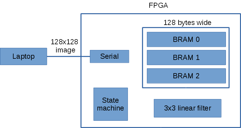
The laptop sends the image over the serial one row at a time to the FPGA. The FPGA then immediately sends the processed pixel row back to the laptop. I chose this design because it only requires three row buffers on the FPGA. The Basys2 has 72Kbits of fast RAM. For an image width of 128 pixels, it only requires 128×3 = 384 bytes of RAM.
The state machine handles all the logic between the serial, BRAM and 3×3 linear filter.
I decided to use serial for communication between the laptop and FPGA because it was simpler, though slower. I did however manage to crank up the serial speed to 1.5 Mbit by adding an external 100Mhz crystal oscillator. Using the default 50Mhz oscillator on the Basys2 I can get up to 1 Mbit.
I use three banks of dual port BRAM (block RAM). The dual port configuration allows two simultaneously read/write to the same BRAM. This allows me to read 3×2=6 pixels in one clock cycle. For 3×3=9 pixels it takes two clock cycles. I could do better by making the read operation return more pixels. The three banks of BRAM act as a circular buffer. There’s some logic in the state machine that keeps track of which bank of BRAM to use for a given input pixel row.
Right now with the my current BRAM configuration and 3×3 filter implementation it takes 5 clock cycles to process a single pixel, excluding serial reading/writing. If you include the serial transmission overhead then it takes about 380 ms on my laptop to process a 128×128 grey image.
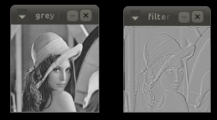
Below is the result of the Laplacian filter on Lena. I ignored the pixels on the border of the image, so the final image is 126×126.
Download
The zip file contains only the necessary Verilog code and a main.cpp for sending the image. The main.cpp requires OpenCV for display. I omitted any Xilinx ISE specific project files to keep it simple. But if there’s any missing files let me know. Your input image must be 128×128 in size to work.
WordPress malware
My site got hit hard with some malicious WordPress trojans (possibly via plugins) and caused the site to get suspended. It’s back up now with a fresh theme. I deleted every plugin and re-installed only the necessary ones. Code highlighting isn’t enabled yet, can’t rememeber what I last installed.
First trip to FPGA land
Been a while since I last posted anything. I’ve been pretty busy at my new job but managed to find some spare time to learn about FPGA. I wanted to see what all the rage is about. I purchased a Digilent Basys2 not too long ago to play with. It’s an entry board under $100, perfect for a noob like myself. Below is the Basys2 board. I bought a serial module so I can communicate using the latop, shown in the top left connected to the red USB cable.

For the first two weeks I went through the digital design book on Digilent’s site to brush up on stuff I should have remembered during my undergrad but didn’t. It’s a pretty good book for a quick intro to the basic building blocks with example code in Verilog/VHDL. I chose the Verilog book over VHDL because I found it easier to read, and less typing.
I then spent the next two or three weeks or so implementing a simple RS232 receiver/transmitter, with help from here. Boy, was that a frustrating project, but I felt I learnt a lot from that experience. That small project helped me learned about RS232 protocol, Verilog, Xilinx ISE and iSim.
Overall, I’m enjoying FPGA land so far despite how difficult it can be. There’s something about being intimately closer to the hardware that I find appealing.
My original intention for learning the FPGA is for image processing and computer vision tasks. The Basys2 doesn’t have a direct interface for a camera so for now I’ll stick to using the serial port to send images as proof of concept. Maybe I’ll upgrade to a board with a camera interface down the track.
I recently wrote a simple 3×3 filter Verilog module to start of with. It’s a discrete 3×3 Laplacian filter.
module filter3x3(
input wire clk,
input wire [7:0] in0,
input wire [7:0] in1,
input wire [7:0] in2,
input wire [7:0] in3,
input wire [7:0] in4,
input wire [7:0] in5,
input wire [7:0] in6,
input wire [7:0] in7,
input wire [7:0] in8,
output reg signed [15:0] q
    );

always @ (posedge clk)
begin
    q <= in0 + in1 + in2 +
          in3 - in4*8 + in5 +
          in6 + in7 + in8;
end

endmodule
This module takes as input 8 unsigned bytes and multiples with the 3×3 kernel [1 1 1; 1 -8 1; 1 1 1] and sums the output to q. It is meant to do this in one clock cycle. I’ve tested it in simulation and it checks out. Next step is to hook up to my serial port module and start filtering images. Stay tune!
Fixing vibration on Taig headstock
I’ve been using the Taig for a few weeks now and had noticed significant vibration on the headstock. I don’t have access to another Taig to compare to see if it’s normal but it definitely “felt” too much. Last week I finally got around to addressing it.
The first thing I noticed was the pulley on the motor being slightly wonky (not running true). After a call to Taig they sent me a replacement pulley. They were very helpful and knowledgeable and know their stuff. They suggested other factors that I can check to help with the vibration issue.
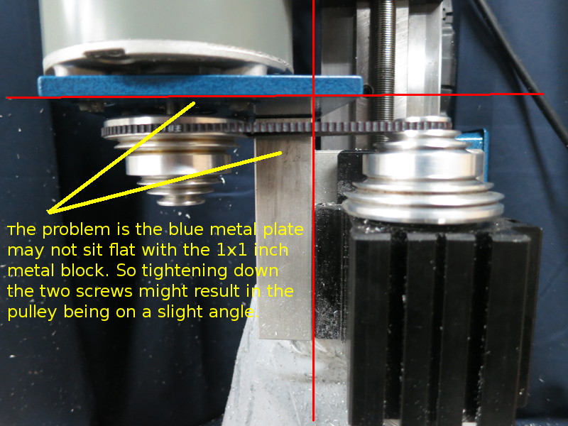
When the pulley arrived I replaced the old one and re-aligned the belt using a parallel and eye balling. Sadly, this did not fix the problem. Then I remember one suggestion by the guys at Taig. He said where the motor mount aligns to the 1×1 inch steel block might not be perfectly flat and could cause vibration because the pulley would be on a slight angle. Guess what, he’s right! With the spindle running at 10,000RPM or so, I applied some force to the motor with my hand and noticed the vibration varied a lot.
This is the hack that I settled on. Every time I adjust the spindle speed I screw the far back screw tight, while the other one is lightly tightened. Just enough so the motor doesn’t twist. I got curious and hooked up a dial indicator to the headstock. As I tightened the screw I could see the vibration ramp up.
Here are two pics that summarize the problem (I think) and the hack fix.
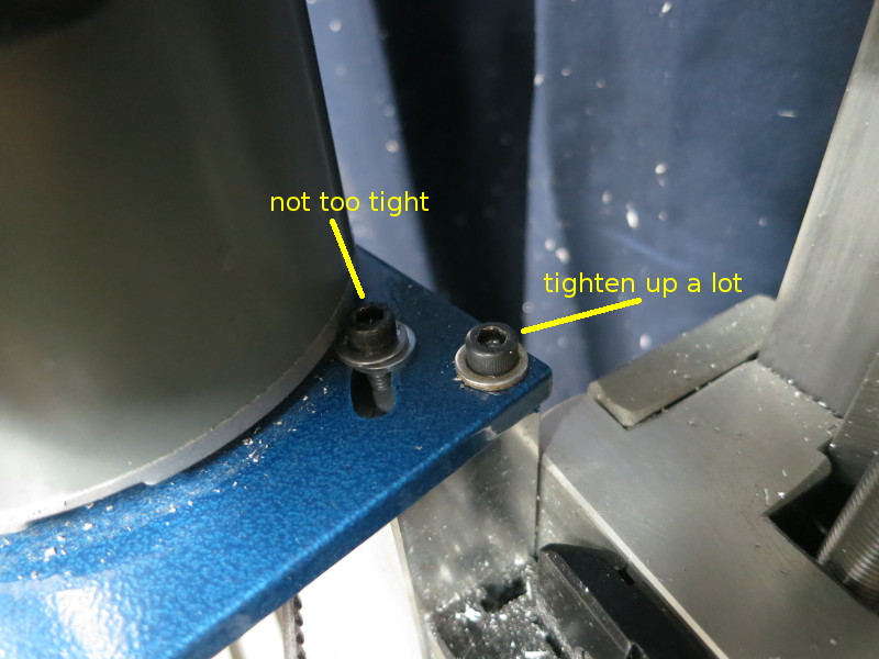
Your situation may differ. Play around with the screws and see what happens.For now it seems to do the job. Vibration is at a minimum, I’m happy.
Machining an aluminium block on the Taig CNC mill
I’ve recently had the chance to get back into some CNC’ing with the Taig CNC mill at work. This is the first time I’ve used the Taig and I must say it’s a pretty slick machine for its size. I was tasked with machining out a rectangular block as an initial step for a more complex part. I thought given how much beefier this CNC is compared to my home made ones it should be a walk in the park. It could not be further from the truth!
I’ve consulted many online/offline calculators and read as much posts from other people’s experience to hone in a setting I was happy with. I’ve lost count of how many end mills I’ve broken along the way! Fortunately I ordered some fairly inexpensive end mills to play with so it wasn’t too bad.
The two most common end mills I’ve used are the 3/8″ 1 inch length of cut and a 1/8″ 1 inch length of cut, both 2 flutes and both from Kodiak. To machine out the block I saved some time by removing most of the material with a drop saw (miter saw). This meant less work for the 3/8″ end mill. Here’s a summary of what I used
3/8″ end mill 2 flutes, 1 inch length of cut
- RPM: ~ 3000
- feed rate: 150 mm/min (~6 ipm)
- plunge rate: 50 mm/min (~2 ipm)
- depth per pass: 2 mm (0.0787″)
1/8″ end mill 2 flutes, 1 inch length of cut
- RPM: ~10,000
- feed rate: 500 mm/min (~20 ipm)
- plunge rate: 200 mm/min
- depth per pass: 0.5 mm (~ 0.02″)
The 1/8″ end mill isn’t used to machine the block but for another job.
Here is my very basic Taig setup. It is bolted to the table top.

There’s no automatic coolant or air flow installed so I’m doing it manually by hand. Not ideal, but does the job and keeps me alert! I’m using Kool Mist 77. That’s the 3/8″ end mill in the pic. It’s about the biggest end mill that is practical on the Taig. I’ve added rubber bands to the safety goggle to stop it from falling off my head because I wear glasses.
Below shows one side of the block I milled. The surface is very smooth to touch.

But when looking on the other side, where the cutter is going in the Y direction it shows some wavy patterns?! Not sure what’s going on there. It didn’t mess up the overall job because it was still smooth enough that I could align it on a vise. Still, would like to know what’s going on.

Here are some things I’ve learnt along the way
Clear those chips!
I originally only used Kool Mist and just squirting extra hard to clear the chips. This got a bit tiring and I wasn’t doing such a great job during deeper cuts. Adding the air hose makes life much easier. I found 20-30 PSI was enough to clear the chips.
Take care when plunging
I’ve read the 2 flutes can handle plunging okay but I always find it struggles if you are not careful. The sound it makes when you plunge can be pretty brutal to the ear, which is why I tend to go conservative. I usually set the plunge rate to half the feed rate and take off 50 mm/min. If I’m doing a job in CamBam I use the spiral plunging option, which does a very gradual plunge while moving the cutter in a spiral. Rather than a straight vertical plunge, which makes it harder to clear chips at the bottom. I’ve broken many smaller end mills doing straight plunges. I once did a plunge with the 3/8″ end mill that was a bit too fast and it completely stalled the motor.
I probably should look at per-drilling holes to minimize plunging.
Go easy!
I’ve found a lot of the answers from the feed rate calculators rather ambitious for the Taig. They tend to assume you got a big ass CNC with crazy horse power. Some of the calculators I’ve used take into consideration the tool deflection and horse power, which is an improvement. But at the end of the day the Taig is a tiny desktop CNC weighing at something like 38kg. So know its limits!
3D camera rig
Been helping out a mate with setting up a 3D camera rig. It’s been a while since I’ve done mechanical work but it’s great to get dirty with machinery again!
Here’s a video of the camera rig being set up. This video is a bit dated, the current setup has lots of lighting stands not shown.
Here’s a result of my head using Agisoft Photocan. Looks pretty good so far!
https://sketchfab.com/models/78c7d06c5d5a482e95032ad0eba7eac2
ICRA 2014 here we come!
Woohoo our paper “Localization on Freeways using the Horizon Line Signature” got accepted for ICRA 2014 Workshop on Visual Place Recognition in Changing Environments! Now I just need to sort out funding. The conference registration is over $1000! Damn, that’s going to hurt my pocket …
This is the new video we’ll be showing at our poster stand
Old school voxel carving
I’ve been working on an old school (circa early 90s) method of creating 3D models called voxel carving. As a first attempt I’m using an academic dataset that comes with camera projection matrices provided. The dataset is from
http://www.cs.wustl.edu/~furukawa/research/mview/index.html
specifically the Predator dataset (I have a thing for Predator).
Here it is in action
Screen recording was done using SimpleScreenRecorder, which was slick and easy to use.
You will need OpenCV installed and the Predator images. Instructions can be found in the README.txt.
Fun with seam cut and graph cut
This fun little project was inspired by a forum post for the Coursera course Discrete Inference and Learning in Artificial Vision.
I use the method outlined in Graphcut Textures: Image and Video Synthesis Using Graph Cuts.
The toy problem is as follows. Given two images overlaid on top of each, with say a 50% overlap, find the best seam cut through the top most image to produce the best “blended” looking image. No actual alpha blending is performed though!
This is a task that can be done physically with two photos and a pair of scissors.
The problem is illustrated with the example below. Here the second image I want to blend with is a duplicate of the first image. The aim is to find a suitable seam cut in the top image such that when I merge the two images it produces the smoothest transition. This may seem unintuitive without alpha blending but it possible depending on the image, not all type of images will work with this method.

By formulating the problem as a graph cut problem we get the following result.

and the actual seam cut in thin red line. You might have to squint.

If you look closely you’ll see some strangeness at the seam, it’s not perfect. But from a distance it’s pretty convincing.
Here are a more examples using the same method as above, that is: duplicate the input image, shift by 50% in the x direction, find the seam cut in the top layer image.


This one is very realistic.
Who likes penguins?


Code
You’ll need OpenCV 2.x install.
I’ve also included the maxflow library from http://vision.csd.uwo.ca/code/ for convenience.
To run call
$ ./SeamCut img.jpg
Simple video stabilization using OpenCV
I’ve been mucking around with video stabilization for the past two weeks after a masters student got me interested in the topic. The algorithm is pretty simple yet produces surprisingly good stabilization for panning videos and forwarding moving (eg. on a motorbike looking ahead). The algorithm works as follows:
- Find the transformation from previous to current frame using optical flow for all frames. The transformation only consists of three parameters: dx, dy, da (angle). Basically, a rigid Euclidean transform, no scaling, no sharing.
- Accumulate the transformations to get the “trajectory” for x, y, angle, at each frame.
- Smooth out the trajectory using a sliding average window. The user defines the window radius, where the radius is the number of frames used for smoothing.
- Create a new transformation such that new_transformation = transformation + (smoothed_trajectory – trajectory).
- Apply the new transformation to the video.
Here’s an example video of the algorithm in action using a smoothing radius of +- 30 frames.
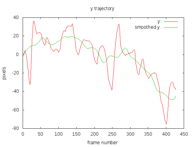
We can see what’s happening under the hood by plotting some graphs for each of the steps mentioned above on the example video.
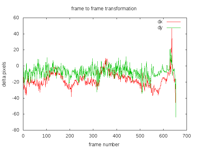
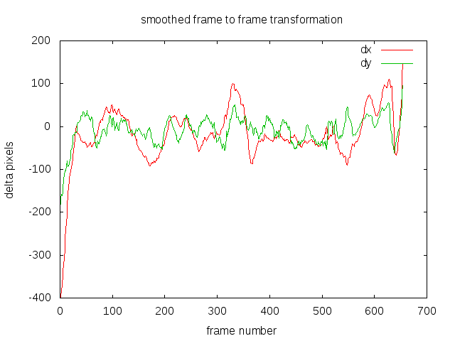
Step 1
This graph shows the dx, dy transformation for previous to current frame, at each frame. I’ve omitted da (angle) because it’s not particularly interesting for this video since there is very little rotation. You can see it’s quite a bumpy graph, which correlates with our observation of the video being shaky, though still orders of magnitude better than Hollywood’s shaky cam effect. I’m looking at you Bourne Supremacy.
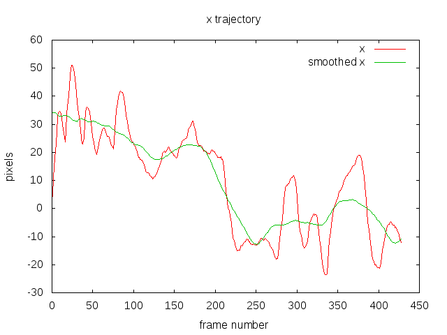
Step 2 and 3
I’ve shown both the accumulated x and y, and their smoothed version so you get a better idea of what the smoothing is doing. The red is the original trajectory and the green is the smoothed trajectory.
It is worth noting that the trajectory is a rather abstract quantity that doesn’t necessarily have a direct relationship to the motion induced by the camera. For a simple panning scene with static objects it probably has a direct relationship with the absolute position of the image but for scenes with a forward moving camera, eg. on a car, then it’s hard to see any.
The important thing is that the trajectory can be smoothed, even if it doesn’t have any physical interpretation.
Step 4
This is the final transformation applied to the video.
Code
videostabKalman.cpp (live version by Chen Jia using a Kalman Filter)
You just need OpenCV 2.x or above.
Once compile run it from the command line via
./videostab input.avi
More videos
Footages I took during my travels.
Project 100k
We (being myself and my buddy Jay) have been working on a fun vision pet project over the past few months. The project started from a little boredom and lots of discussion over wine back in July 2013. We’ve finally got the video done. It demonstrates our vision based localisation system (no GPS) on a car.
The idea is simple, to use the horizon line as a stable feature when performing image matching. The experiments were carried out on the freeway at 80-100 km/h (hence the name of the project). The freeway is just one long straight road, so the problem is simplified and constrained to localisation on a 1D path.
Now without further adieu, the video
We’re hoping to do more work on this project if time permits. The first thing we want to improve on is the motion model. At the moment, the system assumes the car travels at the same speed as the previously collected video (which is true most of the time, but not always eg. bad traffic). We have plans to determine the speed of the vehicle more accurately.
Don’t forget to visit Jay’s website as well !
An old thesis sketch
Here’s an amusing sketch I did for one of my thesis chapter back in November 2008. It was captioned “Concept design of augmented reality system using the vision based localisation”. A friend made it comment it looked like a xkcd drawing.
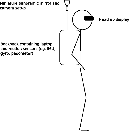
The sketch is pretty crude and funny in hindsight. I originally added it to my thesis to give it an extra “visionary” depth, kind of predicting the future so to speak. I didn’t think anyone would seriously wear such bulky equipment, plus it made you look silly. A few years later Google made this …
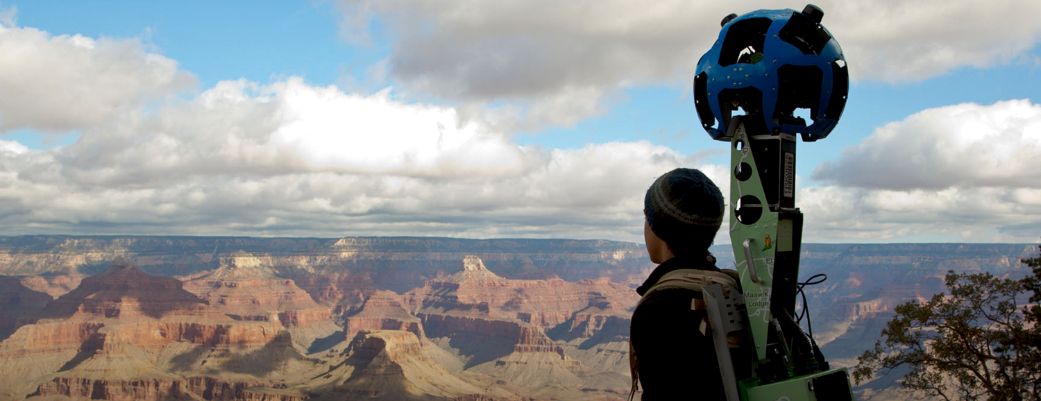
That’s a Google streeview trekker. Different application to what I proposed but the design is not far off!
I should keep a record of all my ideas that I dismiss as impractical and ridiculous. Just so on the off chance someone does implemented it successfully I can get all smug and say I thought of it first 🙂 And then get jealous I didn’t captialise on it …
cppcheck and OpenCV
Every now and then when I’m free and bored, I do a daily git fetch on the OpenCV branch to keep up to date with the latest and greatest. One of my favourite things to do is run cppcheck on the source code to see what new bugs have appeared (I should find a new hobby). For those who don’t know what cppcheck is, it is an open source static code analyzer for C/C++. It will try to find coding mistakes eg. using an uinitialised variable, memory leak, and more. In other words, it is a must have tool, use it, and use it often.
To demonstrate its effectiveness, I just updated my OpenCV 2.4 branch as of 15th Dec 2013 and ran cppcheck on it, resulting in:
$ cppcheck -q -j 4 .
[features2d/src/orb.cpp:179]: (error) Uninitialized variable: ix
[features2d/src/orb.cpp:199]: (error) Uninitialized variable: ix
[features2d/src/orb.cpp:235]: (error) Uninitialized variable: ix
[features2d/src/orb.cpp:179]: (error) Uninitialized variable: iy
[features2d/src/orb.cpp:199]: (error) Uninitialized variable: iy
[features2d/src/orb.cpp:235]: (error) Uninitialized variable: iy
[imgproc/src/color.cpp:773]: (error) Array 'coeffs[2]' accessed at index 2, which is out of bounds.
[imgproc/test/test_cvtyuv.cpp:590]: (style) Class 'ConversionYUV' is unsafe, 'ConversionYUV::yuvReader_' can leak by wrong usage.
[imgproc/test/test_cvtyuv.cpp:591]: (style) Class 'ConversionYUV' is unsafe, 'ConversionYUV::yuvWriter_' can leak by wrong usage.
[imgproc/test/test_cvtyuv.cpp:592]: (style) Class 'ConversionYUV' is unsafe, 'ConversionYUV::rgbReader_' can leak by wrong usage.
[imgproc/test/test_cvtyuv.cpp:593]: (style) Class 'ConversionYUV' is unsafe, 'ConversionYUV::rgbWriter_' can leak by wrong usage.
[imgproc/test/test_cvtyuv.cpp:594]: (style) Class 'ConversionYUV' is unsafe, 'ConversionYUV::grayWriter_' can leak by wrong usage.
[legacy/src/calibfilter.cpp:725]: (error) Resource leak: f
[legacy/src/epilines.cpp:3005]: (error) Memory leak: objectPoints_64d
[legacy/src/epilines.cpp:3005]: (error) Memory leak: rotMatrs1_64d
[legacy/src/epilines.cpp:3005]: (error) Memory leak: rotMatrs2_64d
[legacy/src/epilines.cpp:3005]: (error) Memory leak: transVects1_64d
[legacy/src/epilines.cpp:3005]: (error) Memory leak: transVects2_64d
[legacy/src/vecfacetracking.cpp] -> [legacy/src/vecfacetracking.cpp:670]: (error) Internal error. Token::Match called with varid 0. Please report this to Cppcheck developers
[ml/src/svm.cpp:1338]: (error) Possible null pointer dereference: df
[objdetect/src/hog.cpp:2564]: (error) Resource leak: modelfl
: (error) Division by zero.
[ts/src/ts_gtest.cpp:7518]: (error) Address of local auto-variable assigned to a function parameter.
[ts/src/ts_gtest.cpp:7518]: (error) Uninitialized variable: dummy
[ts/src/ts_gtest.cpp:7525]: (error) Uninitialized variable: dummy
cppcheck -q – j 4, calls cppcheck in quiet mode (only reporting errors) using 4 threads.
The orb.cpp errors are fairly new. The others have been there for a while because I didn’t bother sending a pull request for the legacy functions, because well, they’re legacy. But I should.
The error in tvl1flow.cpp is a false alert, which I’ve reported and has been resolved. Basically, someone used a variable called div, which cppcheck confuses with the stdlib.h div function, because they both have the same parameter count and type, naughty.
vecfecetracking.cpp is an interesting one, cppcheck basically failed for some unknown reason. Though it rarely occurs. I should report that to the cppcheck team.
hog.cpp reports a resource leak because an fopen was called prior but the function calls a throw if something goes wrong without calling fclose, as shown below:
void HOGDescriptor::readALTModel(std::string modelfile)
{
   // read model from SVMlight format..
   FILE *modelfl;
   if ((modelfl = fopen(modelfile.c_str(), "rb")) == NULL)
   {
       std::string eerr("file not exist");
       std::string efile(__FILE__);
       std::string efunc(__FUNCTION__);
       throw Exception(CV_StsError, eerr, efile, efunc, __LINE__);
   }
   char version_buffer[10];
   if (!fread (&version_buffer,sizeof(char),10,modelfl))
   {
       std::string eerr("version?");
       std::string efile(__FILE__);
       std::string efunc(__FUNCTION__);
       // doing an fclose(modefl) would fix the error
       throw Exception(CV_StsError, eerr, efile, efunc, __LINE__);
   }
With holidays coming up in a week I’ll probably get off my lazy ass and submit some more fixes. What I find funny is the fact that I’ve been seeing the same errors for the past months (years even?). It seems to suggest cppcheck needs to be publicised more and possibly become part of the code submission guideline. I feel like I’m the only one running cppcheck on OpenCV.
UPDATE:
Running with the latest cppcheck 1.62 produces less false alerts than before (was running 1.61). I now get:
[highgui/src/cap_images.cpp:197]: (warning) %u in format string (no. 1) requires 'unsigned int *' but the argument type is 'int *'.
[imgproc/test/test_cvtyuv.cpp:590]: (style) Class 'ConversionYUV' is unsafe, 'ConversionYUV::yuvReader_' can leak by wrong usage.
[imgproc/test/test_cvtyuv.cpp:591]: (style) Class 'ConversionYUV' is unsafe, 'ConversionYUV::yuvWriter_' can leak by wrong usage.
[imgproc/test/test_cvtyuv.cpp:592]: (style) Class 'ConversionYUV' is unsafe, 'ConversionYUV::rgbReader_' can leak by wrong usage.
[imgproc/test/test_cvtyuv.cpp:593]: (style) Class 'ConversionYUV' is unsafe, 'ConversionYUV::rgbWriter_' can leak by wrong usage.
[imgproc/test/test_cvtyuv.cpp:594]: (style) Class 'ConversionYUV' is unsafe, 'ConversionYUV::grayWriter_' can leak by wrong usage.
[legacy/src/calibfilter.cpp:725]: (error) Resource leak: f
[legacy/src/epilines.cpp:3005]: (error) Memory leak: objectPoints_64d
[legacy/src/epilines.cpp:3005]: (error) Memory leak: rotMatrs1_64d
[legacy/src/epilines.cpp:3005]: (error) Memory leak: rotMatrs2_64d
[legacy/src/epilines.cpp:3005]: (error) Memory leak: transVects1_64d
[legacy/src/epilines.cpp:3005]: (error) Memory leak: transVects2_64d
[ml/src/svm.cpp:1338]: (error) Possible null pointer dereference: df
[objdetect/src/hog.cpp:2564]: (error) Resource leak: modelfl
[ts/src/ts_gtest.cpp:7518]: (error) Address of local auto-variable assigned to a function parameter.
[ts/src/ts_gtest.cpp:7518]: (error) Uninitialized variable: dummy
[ts/src/ts_gtest.cpp:7525]: (error) Uninitialized variable: dummy
Haar wavelet denoising
This is some old Haar wavelet code I dug up from my PhD days that I’ve adapted to image denoising. It denoises an image by performing the following steps
- Pad the width/height so the dimensions are a power of two. Padded with 0.
- Do 2D Haar wavelet transform
- Shrink all the coefficients using the soft thresholding: x = sign(x) * max(0, abs(x) – threshold)
- Inverse 2D Haar wavelet transform
- Remove the padding
I’ve coded a simple GUI using OpenCV to show the denoising in action. There’s a slider that goes from 0 to 100, which translates to a threshold range of [0, 0.1].
I’ll use the same image in a previous post. This is a cropped image taken at night on a point and shoot camera. The noise is real and not artificially added.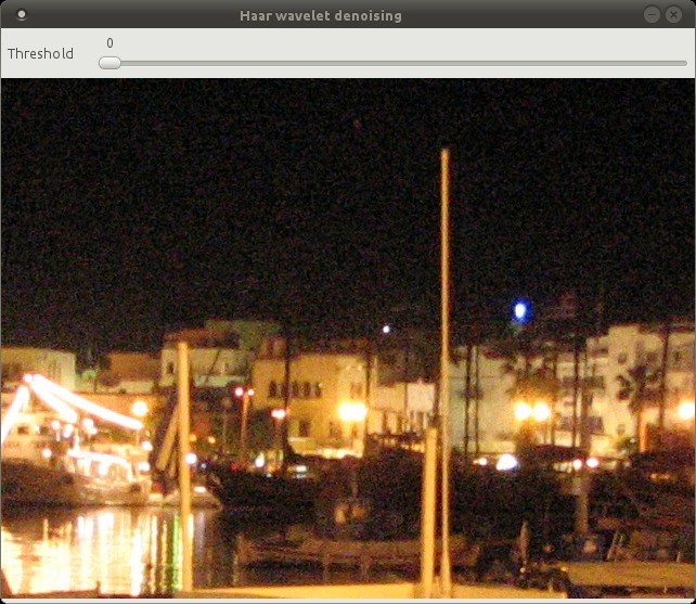
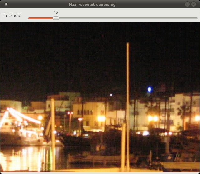
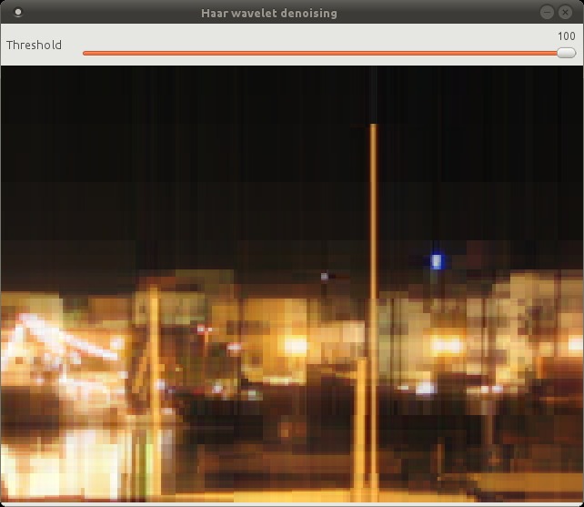
The Haar wavelet does a pretty good job of preserving edges and sharp transitions in general. At threshold = 100 you start to see the blocky nature of the Haar wavelet.
One downside of using the Haar wavelet is that the image dimensions have to be a power of two, which wastes memory and CPU cycles when we have to pad the image.
Download
Compile using GCC with
g++ haar_wavelet_denoising.cpp -o haar_wavelet_denoising -O3 -lopencv_core -lopencv_highgui -lopencv_imgproc
and run via
./haar_wavelet_denoising image.jpg
Asimo Vitruvian Man project
Had a busy weekend crafting this small gift of appreciation for our PhD supervisor. The design was a collaborative effort with my colleagues. The base features an Asimo version of Da Vinci’s Vitruvian Man. It took us from 10.30 am to 5.30 pm to complete the base due to a lot of filing/sanding (tool wasn’t sharp enough) and design changes along the way. The Asimo figured was 3D printed by Jay and took about 5 hours. Overall, everything was completed from start to finish within 5 days, after many many many email exchanges between us.


Convolutional neural network and CIFAR-10, part 3
This is a continuation from the last post. This time I implemented translation + horizontal flipping. The translation works by cropping the 32×32 image into smaller 24×24 sub-images (9 to be exact) to expand the training set and avoid over fitting.
This is the network I used
- Layer 1 – 5×5 Rectified Linear Unit, 64 output maps
- Layer 2 – 2×2 Max-pool
- Layer 3 – 5×5 Rectified Linear Unit, 64 output maps
- Layer 4 – 2×2 Max-pool
- Layer 5 – 3×3 Rectified Linear Unit, 64 output maps
- Layer 6 – Fully connected Rectified Linear Unit, 64 output neurons
- Layer 7 – Fully connected linear units, 10 output neurons
- Layer 8 – Softmax
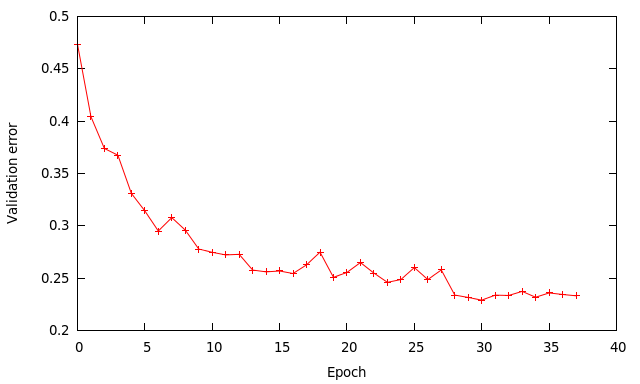
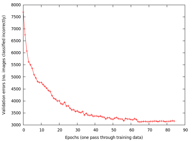
Below is the validation error during training. I’ve changed the way the training data is loaded to save memory. Each dataset is loaded and trained one at a time, instead of loading it all into memory. After a dataset is trained I output the validation error to file. Since I use 4 datasets for training each data point on the graph represents 1/4 of an epoch (one pass through all the training data).
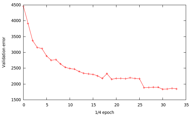
I used an initial learning rate of 0.01, then changed to 0.001 at x=26 then finally 0.0001 at x=30. The other training parameters are
- momentum = 0.9
- mini batch size = 64
- all the data centred (mean subtracted) prior to training
- all weights initialised using a Gaussian of u=0 and stdev=0.1 (for some reason it doesn’t work with 0.01 like most people do)
The final results are:
- training error ~ 17.3%
- validation error ~ 18.5%
- testing error ~ 20.1%
My last testing error was 24.4% so there is some slight improvement, though at the cost of much more computation. The classification code has been modified to better suit the 24×24 cropped sub-images. Rather than classify using only the centre sub-image all 9 sub-images are used. The softmax results from each sub-image is accumulated and the highest score picked. This works much better than using the centre image only. This is idea is borrowed from cuda-convnet.
Here are the features learnt for the first layer.
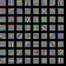
Using cropped sub-images and horizontal flipping the training set has expanded 18 times. The error gap between training error and validation error is now much smaller than before. This suggests I can gain improvements by using a neural network with a larger modeling capacity. This is true for the network used by cuda-convnet to get < 13% training error. Their network is more complex than what I’m using to achieve those results. This seems to be a ‘thing’ with neural networks where to get that extra bit of oomph the complexity of the network can grow monstrously, which is rather off putting.
Based on results collected for the CIFAR-10 dataset by this blog post the current best is using something called a Multi-Column Deep Neural Network, which achieves an error of 11.21%. It uses 8 different convolution neural networks (dubbed ‘column’) and aggregate the results together (like a random forest?). Each column receives the original RGB images plus some pre-processed variations. The individual neural network column themselves are fairly big beasts consisting of 10 layers.
I think there should be a new metric (or maybe there already is) along the lines of “best bangs for bucks”, where the state of the art algorithms are ranked based on something like [accuracy]/[number of model parameters], which is of particular interest in resource limited applications.
Download
To compile and run this code you’ll need
- CodeBlocks
- OpenCV 2.x
- CUDA SDK
- C++ compiler that supports the newer C++11 stuff, like GCC
Instructions are in the README.txt file.
Convolutional neural network and CIFAR-10, part 2
Spent like the last 2 weeks trying to find a bug in the code that prevented it from learning. Somehow it miraculously works now but I haven’t been able to figure out why. First thing I did immediately was commit it to my private git in case I messed it up again. I’ve also ordered a new laptop to replace my non-gracefully aging Asus laptop with a Clevo/Sager, which sports a GTX 765M. Never tried this brand before, crossing my fingers I won’t have any problems within 2 years of purchase, unlike every other laptop I’ve had …
I’ve gotten better results now by using a slightly different architecture than before. But what improved performance noticeably was increasing the training samples by generating mirrored versions, effectively doubling the size. Here’s the architecture I used
Layer 1 – 5×5 convolution, Rectified Linear units, 32 output channels
Layer 2 – Average pool, 2×2
Layer 3 – 5×5 convolution, Rectified Linear units, 32 output channels
Layer 4 – Average pool, 2×2
Layer 5 – 4×4 convolution, Rectified Linear units, 64 output channels
Layer 6 – Average pool, 2×2
Layer 7 – Hidden layer, Rectified Linear units, 64 output neurons
Layer 8 – Hidden layer, Linear units, 10 output neurons
Layer 9 – Softmax
The training parameters changed a bit as well:
- learning rate = 0.01, changed to 0.001 at epoch 28
- momentum = 0.9
- mini batch size = 64
- all weights initialised using a Gaussian of u=0 and stdev=0.1
For some reason my network is very sensitive to the weights initialised. If I use a stdev=0.01, the network simply does not learn at all, constant error of 90% (basically random chance). My first guess is maybe something to do with 32bit floating point precision, particularly when small numbers keep getting multiply with other smaller numbers as they pass through each layer.
 The higher learning rate of 0.01 works quite well and speeds up the learning process compared to using a rate of 0.001 I used previously. Using a batch size of 64 instead of 128 means I perform twice as many updates per epoch, which should be a good thing. A mini batch of 128 in theory should give a smoother gradient than 64 but since we’re doing twice as many updates it sort of compensates.
At epoch 28 I reduce the learning rate to 0.001 to get a bit more improvement. The final results are:
- training error – 9%
- validation error – 23.3%
- testing error – 24.4%
The results are similar to the ones by cuda-convnet for that kind of architecture. The training error being much lower than the other values indicates the network has enough capacity to model most of the data, but is limited by how well it generalises to unseen data.
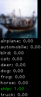
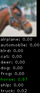
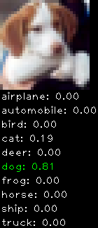
Numbers alone are a bit boring to look at so I thought it’d be cool to see visually how the classifier performs. I’ve made it output 20 correct/incorrect classifications on the test datase4t with the probability of it belonging to a particular category (10 total).
Correctly classified
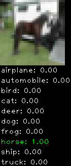
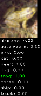
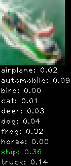
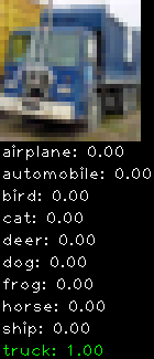
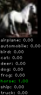
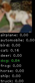
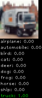
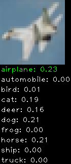
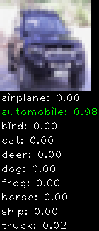
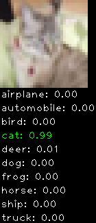
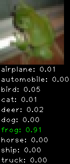
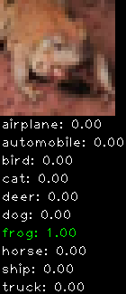

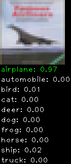
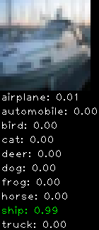
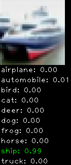
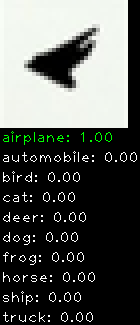
Incorrectly classified
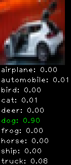
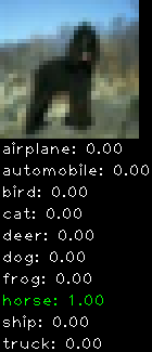
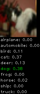
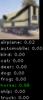

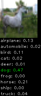
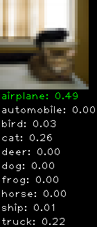
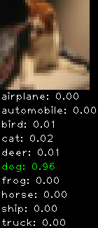
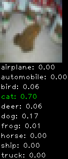
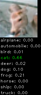

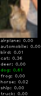
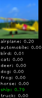
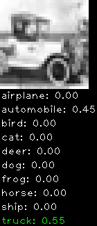
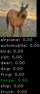
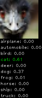
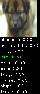
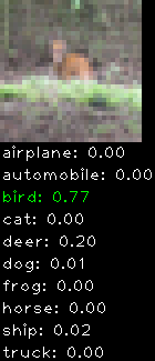
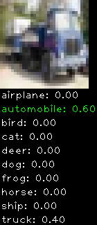
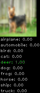
The miss classification are interesting because it gives us some idea what trips up the neural network. For example, the animals tend to get mix up a bit because they share similar physical characteristics eg. eyes, legs, body.
Next thing I’ll try is to add translated versions of the training data. This is done by cropping the original 32×32 image into say 9 overlapping 24×24 images, evenly sampled. For each of the cropped images we can mirror them as well. This improves robustness to translation and has been reported to give a big boost in classification accuracy. It’ll expand the training data up to 18 times (9 images, plus mirror) ! Going to take a while to run …
I’m also in the process of cleaning the code. Not sure on a release date, if ever. There are probably better implementation of convolutional neural network (EBlearn, cuda-convnet) out there but if you’re really keen to use my code leave a comment below.
Convolutional neural network and CIFAR-10
I’ve been experimenting with convolutional neural networks (CNN) for the past few months or so on the CIFAR-10 dataset (object recognition). CNN have been around since the 90s but seem to be getting more attention ever since ‘deep learning’ became a hot new buzzword.
Most of my time was spent learning the architecture and writing my own code so I could understand them better. My first attempt was a CPU version, which worked correctly but was not fast enough for any serious use. CNN with complex architectures are notoriously slow to train, that’s why everyone these days use the GPU. It wasn’t until recently that I got a CUDA version of my code up and running. To keep things simple I didn’t do any fancy optimisation. In fact, I didn’t even use shared memory, mostly due to the way I structured my algorithm. Despite that, it was about 10-11x faster than the CPU version (single thread). But hang on, there’s already an excellent CUDA CNN code on the net, namely cuda-convnet, why bother rolling out my own one? Well, because my GPU is a laptop GTS 360M (circa 2010 laptop), which only supports CUDA compute 1.2. Well below the minimum requirements of cuda-convnet. I could get a new computer but where’s the fun in that 🙂 And also, it’s fun to re-invent the wheel for learning reasons.
Results
As mentioned previously I’m working with the CIFAR-10 dataset, which has 50,000 training images and 10,000 test images. Each image is a tiny 32×32 RGB image. I split the 50,000 training images into 40,000 and 10,000 for training and validation, respectively. The dataset has 10 categories ranging from dogs, cats, cars, planes …
The images were pre-processed by subtracting each image by the average image over the whole training set, to centre the data.
The architecture I used was inspired from cuda-convnet and is
Input – 32×32 image, 3 channels
Layer 1 – 5×5 convolution filter, 32 output channels/features, Rectified Linear Unit neurons
Layer 2 – 2×2 max pool, non-overlapping
Layer 3 – 5×5 convolution filter, 32 output channels/features, Rectified Linear Unit neurons
Layer 4 – 2×2 max pool, non-overlapping
Layer 5 – 5×5 convolution filter, 64 output channels/features, Rectified Linear Unit neurons
Layer 6 – fully connected neural network hidden layer, 64 output units, Rectified Linear Unit neurons
Layer 7 – fully connected neural network hidden layer, 10 output units, linear neurons
Layer 8 – softmax, 10 outputs
I trained using a mini-batch of 128, with a learning rate of 0.001 and momentum of 0.9. At each epoch (one pass through the training data), the data is randomly shuffled. At around the 62th epoch I reduced the learning rate to 0.0001. The weights are updated for each mini-batch processed. Below shows the validation errors vs epoch.
After 85 epochs the results are:
– training error 7995/40000 ~ 20%
– validation error 3156/10000 = 31.56%
– test error 3114/10000 = 31.14%
Results seem okay until I compared them with results reported by cuda-convnet simplest architecture [1] [2]: ~8 epochs (?), 80 seconds, 26% testing error. Where as mine took a few hours and many more epochs, clearly I’m doing something wrong!!! But what? I did a rough back of the envelope calculation and determined that their GPU code runs 33x faster than mine, based on timing values they reported. Which means my CUDA code and hardware sucks badly.
On the plus side I did manage to generate some cool visualisation of the weights for layer 1. These are the convolution filters it learnt. This result is typical of what you will find published in the literature, so I’m confident I’m doing something right.
You can see it has learnt some edge and colour filters.
One thing I really want to try at the moment is to get my hands on a newer Nvidia card and see how much speed up I get without doing anything to the code.
I’m not releasing any code yet because it’s very experimental and too ugly to show.
Octave’s amusing fact() function
Using Octave today I was taking a guess at the function for factorial might be fact() only to find this amusing snippet:
— Command: fact
— Function File: T = fact()
Display an amazing and random fact about the world’s greatest
hacker.
Running it a few time came up with Chuck Norris equivalent jokes for Richard Stallman:
octave:4> fact

When Richard Stallman executes ps -e, you show up.

octave:5> fact

Richad Stallman's pinky finger is really a USB memory stick.

octave:6> fact

Richard Stallman discovered extra-terrestrial life but killed them because they
used non-free software.

octave:7> fact

Behind Richard Stallman's beard there is another fist, to code faster.

octave:8> fact

Richard Stallman's doesn't kill a process, he just dares it to stay running.
That’s pretty cute.
Sparse model denoising in action
I would like to share some denoising results using sparse modelling based on the SPAMS package. This was inspired by the topic of sparse modeling from the course ‘Image and video processing: From Mars to Hollywood with a stop at the hospital’ at Coursera. I highly recommend this course because it presents some state of the art methods in computer vision that I would have missed otherwise.
I was interested to see how well it would work on real noisy images so I found an old photo I took using a Canon Powershot S3 shot at night on 1600 ISO. Here is a 100% crop of the photo. As you can see, the noise is pretty awful!

Since there is a black sky in the background I thought it’ll be interesting to see what the noise distribution looks like. What do you know, it’s very Gaussian like! This is great because the square error formulation is well suited to this type of noise.

There are a few sparse model parameters one can fiddle around with, but in my experiement I’ve the kept the following fixed and only adjusted lambda since it seems to have the most pronounced effect
- K = 200, dictionary size (number of atoms)
- iterations = 100 – Ithink it’s used to optimize the dictionary + sparse vector
- patch size = 8 (8×8 patch)
- patch stride = 2 (skip every 2 pixels)
Here is with lambda = 0.1

lambda = 0.2

lambda = 0.9

It’s amazing how well it preserves the detail, especially the edges.
Python code can be downloaded here denoise.py_ (right click save as and remove the trailing _)
RBM and sparsity penalty
This is a follow up on my last post about trying to use RBM to extract meaningful visual features. I’ve been experimenting with a sparsity penalty that encourages the hidden units to rarely activate. I had a look at ‘A Practical Guide to Training Restricted Boltzmann Machines’ for some inspiration but had trouble figuring out how their derived formula fits into the training process. I also found some interesting discussions on MetaOptimize pointing to various implementations. But in the end I went for a simple approach and used the tools I learnt from the Coursera course.
The sparsity is the average probability of a unit being active, so they are applicable to sigmoid/logistic units. For my RBM this will be the hidden layer. If you look back in my previous post you can see the weights generate random visual patterns. The hidden units are active about 50% of the time, hence the random looking pattern.
What we want to do is reduce the sparsity so that the units are activated on average a small percentage of the time, which we’ll call the ‘target sparsity’. Using a typical square error, we can formulate the penalty as:
^2")
\right)")
- K is a constant multiplier to tune the gradient step.
- s is the current sparsity and is a scalar value, it is the average of all the MxN matrix elements.
- t is the target sparsity, between [0,1].
Let the forward pass starting from the visible layer to the hidden layer be:

")

- w is the weight matrix
- x is the data matrix
- b is the bias vector
- z is the input to the hidden layer
The derivative of the sparsity penalty, p, with respect to the weights, w, using the chain rule is:

The derivatives are:
 \;\; \leftarrow scalar")

")

The derivative of the sparsity penalty with respect to the bias is the same as above except the last partial derivative is replaced with:

In actual implementation I omitted the constant 
Results
I used an RBM with the following settings:
- 5000 input images, normalized to
- no. of visible units (linear) = 64 (16×16 greyscale images from the CIFAR the database)
- no. of hidden units (sigmoid) = 100
- sparsity target = 0.01 (1%)
- sparsity multiplier K = 1.0
- batch training size = 100
- iterations = 1000
- momentum = 0.9
- learning rate = 0.05
- weight refinement using an autoencoder with 500 iterations and a learning rate of 0.01

and this is what I got
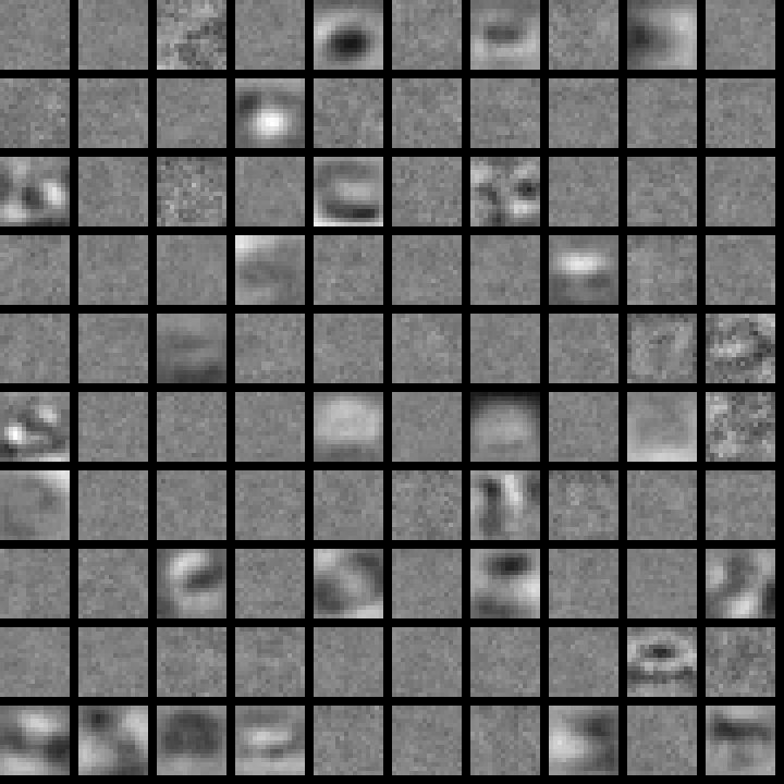 Quite a large portion of the weights are nearly zerod out. The remaining ones have managed to learn a general contrast pattern. It’s interesting to see how smooth they are. I wonder if there is an implicit L2 weight decay, like we saw in the previous post, from introducing the sparsity penalty. There are also some patterns that look like they’re still forming but not quite finished.
The results are certainly encouraging but there might be an efficiency drawback. Seeing as a lot of the weights are zeroed out, it means we have to use more hidden units in the hope of finding more meaningful patterns. If I keep the same number of units but increase the sparsity target then it approaches the random like patterns.
Download
Have a look at the README.txt for instructions on obtaining the CIFAR dataset.
RBM, L1 vs L2 weight decay penalty for images
I’ve been fascinated for the past months or so on using RBM (restricted Boltzmann machine) to automatically learn visual features, as oppose to hand crafting them. Alex Krizhevsky’s master thesis, Learning Multiple Layers of Features from Tiny Images, is a good source on this topic. I’ve been attempting to replicate the results on a much smaller set of data with mix results. However, as a by product of I did manage generate some interesting results.
One of the tunable parameters of an RBM (neural network as well) is a weight decay penalty. This regularisation penalises large weight coefficients to avoid over-fitting (used conjunction with a validation set). Two commonly used penalties are L1 and L2, expressed as follows:


where theta is the coefficents of the weight matrix.
L1 penalises the absolute value and L2 the squared value. L1 will generally push a lot of the weights to be exactly zero while allowing some to grow large. L2 on the other hand tends to drive all the weights to smaller values.
Experiment
To see the effect of the two penalties I’ll be using a single RBM with the following configuration:
- 5000 input images, normalized to
- no. of visible units (linear) = 64 (16×16 greyscale images from the CIFAR the database)
- no. of hidden units (sigmoid) = 100
- batch training size = 100
- iterations = 1000
- momentum = 0.9
- learning rate = 0.01
- weight refinement using an autoencoder with 500 iterations and learning rate of 0.01

The weight refinement step uses a 64-100-64 autoencoder with standard backpropagation.
Results
For reference, here are the 100 hidden layer patterns without any weight decay applied:
 As you can see they’re pretty random and meaningless There’s no obvious structure. Though what is amazing is that even with such random patterns you can reconstruct the original 5000 input images quite well using a weighted linear combinations of them.
Now applying an L1 weight decay with a weight decay multiplier of 0.01 (which gets multiplied with the learning rate) we get something more interesting:
 We get stronger localised “spot” like features.
And lastly, applying L2 weight decay with a multiplier of 0.1 we get
 which again looks like a bunch of random patterns except smoother. This has the effect of smoothing the reconstruction image.
Despite some interesting looking patterns I haven’t really observed the edge or Gabor like patterns reported in the literature. Maybe my training data is too small? Need to spend some more time …
HP Pavilion DM1 + AMD E-450 APU, you both suck!
Last year I bought myself a small HP Pavilion DM1 for traveling overseas. On paper the specs look great compared to any of Asus EEE PC offering in terms of processing power and consumption. It’s got a dual core AMD E-450, Radeon graphics card, 2GB RAM and about 4-5 hrs of battery life. In reality? I’ve had to take this laptop in for warranty repair TWICE in a few short months. First time was a busted graphics chip that only worked if I plugged in an external monitor. The second time was a faulty hard disk singing the click of the death. Both were repaired within a day, so I can’t get too mad. But when I finally got around to installing all the tools I need to do some number crunching under Linux, this happens …
 Yes that’s right, Octave crashes on a matrix multiply!!! WTF?!?
I ran another program I wrote in GDB and it reveals this interesting snippet

My guess is it’s trying to call some AMD assembly instruction that doesn’t exist on this CPU. Octave uses /usr/lib/libblas as well, which explains the crash earlier. Oh well, bug report time …
RBM Autoencoders
I’ve just finished the wonderful “Neural Networks for Machine Learning” course on Coursera and wanted to apply what I learnt (or what I think I learnt). One of the topic that I found fascinating was an autoencoder neural network. This is a type of neural network that can “compress” data similar to PCA. An example of the network topology is shown below.

The network is fully connected and symmetrical, but I’m too lazy to draw all the connections. Given some input data the network will try to reconstruct it as best as it can on the output. The ‘compression’ is controlled mainly by the middle bottleneck layer. The above example has 8 input neurons, which gets squashed to 4 then to 2. I will use the notation 8-4-2-4-8 to describe the above autoencoder networks.
An autoencoder has the potential to do a better job of PCA for dimensionality reduction, especially for visualisation since it is non-linear.
My autoencoder
I’ve implemented a simple autoencoder that uses RBM (restricted Boltzmann machine) to initialise the network to sensible weights and refine it further using standard backpropagation. I also added common improvements like momentum and early termination to speed up training.
I used the CIFAR-10 dataset to train 100 small images of dogs. The images are 32×32 (1024 vector) colour images, which I converted to grescale. The network I train on is:
1024-256-64-8-64-256-1024
The input, output and bottleneck are linear with the rest being sigmoid units. I expected this autoencoder to reconstruct the image better than PCA, because it has much more parameters. I’ll compare the results with PCA using the first 8 principal components.
Results
Here are 10 random results from the 100 images I trained on.


The autoencoder does indeed give a better reconstruction than PCA. This gives me confidence that my implementation is somewhat correct.
The RMSE (root mean squared error) for the autoencoder is 9.298, where as for PCA it is 30.716, pixel values range from [0,255].
All the parameters used can be found in the code.
Download
You can download the code here
Last update: 27/07/2013
You’ll need the following libraries installed
- Armadillo (http://arma.sourceforge.net)
- OpenBLAS (or any other BLAS alternative, but you’ll need to edit the Makefile/Codeblocks project)
- OpenCV (for display)
On Ubuntu 12.10 I use the OpenBLAS package in the repo. Use the latest Armadillo from the website if the Ubuntu one doesn’t work, I use some newer function introduced recently. I recommend using OpenBLAS over Atlas with Armadillo on Ubuntu 12.10, because multi-core support works straight out of the box. This provides a big speed up.
You’ll also need the dataset http://www.cs.toronto.edu/~kriz/cifar-10-binary.tar.gz
Edit main.cpp and change DATASET_FILE to point to your CIFAR dataset path. Compile via make or using CodeBlocks.
All parameter variables can be found in main.cpp near the top of the file.
OpenCV vs. Armadillo vs. Eigen vs. more! Round 3: pseudoinverse test
Okay, the title of this post is getting longer and sillier, but this is the 3rd continuation of my last two post on comparing different libraries for everyday matrix operations. The last two posts compared basic operations such as multiplication, transposition, inversion etc. etc. in isolation, which is probably not a good reflection of real life usage. So I decided to come up with a new test that would combine different matrix operations together. I chose the pseudoinverse because it is something I use every now and then and it combines multiplication, transposition and inversion, which seems like a good test.
For benchmarking I’m going to be solving the following over determined linear system:

and solve for X using
^{-1}A^{T}B")
A is a NxM matrix, where N is much larger than M. I’ll be using N=1,000,000 data points and M (dimensions of the data) varying from 2 to 16.
B is a Nx1 matrix.
The matrix values will be randomly generated from 0 to 1 with uniform noise of [-1,1] added to B. They values are kept to a small range to avoid any significant numerical problems that can come about doing the pseudoinverse this way, not that I care too much for this benchmark. Each test is performed for 10 iterations, but not averaged out since I’m not interested in absolute time but relative to the other libraries.
Just to make the benchmark more interesting I’ve added GSL and OpenBLAS to the test, since they were just an apt-get away on Ubuntu.
Results
The following libraries were used
- OpenCV 2.4.3 (compiled from source)
- Eigen 3.1.2 (C++ headers from website)
- Armadillo 3.4.4 (compiled from source)
- GSL 1.15 (Ubuntu 12.10 package)
- OpenBLAS 1.13 (Ubuntu 12.10 package)
- Atlas 3.8.4 (Ubuntu 12.10 package)
My laptop has an Intel i7 1.60GHz with 6GB of RAM.
All values reported are in milliseconds. Each psuedoinverse test is performed 10 times but NOT averaged out. Lower is better. Just as a reminder each test is dealing with 1,000,000 data points of varying dimensions.
| 2 | 3 | 4 | 5 | 6 | 7 | 8 | 9 | |
| OpenCV | 169.619 | 321.204 | 376.3 | 610.043 | 873.379 | 1185.82 | 1194.12 | 1569.16 |
| Eigen | 152.159 | 258.069 | 253.844 | 371.627 | 423.474 | 577.065 | 555.305 | 744.016 |
| Armadillo + Atlas | 162.332 | 184.834 | 273.822 | 396.629 | 528.831 | 706.238 | 848.51 | 1088.47 |
| Armadillo + OpenBLAS | 79.803 | 118.718 | 147.714 | 298.839 | 372.235 | 484.864 | 411.337 | 507.84 |
| GSL | 507.052 | 787.429 | 1102.07 | 1476.67 | 1866.33 | 2321.66 | 2831.36 | 3237.67 |
| 10 | 11 | 12 | 13 | 14 | 15 | 16 | |
| OpenCV | 1965.95 | 2539.57 | 2495.63 | 2909.9 | 3518.22 | 4023.67 | 4064.92 |
| Eigen | 814.683 | 1035.96 | 993.226 | 1254.8 | 1362.02 | 1632.31 | 1615.69 |
| Armadillo + Atlas | 1297.01 | 1519.04 | 1792.74 | 2064.77 | 1438.16 | 1720.64 | 1906.79 |
| Armadillo + OpenBLAS | 534.947 | 581.294 | 639.175 | 772.382 | 824.971 | 825.79 | 893.771 |
| GSL | 3778.44 | 4427.47 | 4917.54 | 6037.29 | 6303.08 | 7187.5 | 7280.27 |
Ranking from best to worse
- Armadillo + OpenBLAS
- Eigen
- Armadillo + Atlas (no multi-core support out of the box???)
- OpenCV
- GSL
All I can say is, holly smokes Batman! Armadillo + OpenBLAS wins out for every single dimension! Last is GSL, okay no surprise there for me. It never boasted being the fastest car on the track.
The cool thing about Armadillo is switching the BLAS engine only requires a different library to be linked, no recompilation of Armadillo. What is surprising is the Atlas library doesn’t seem to support multi-core by default. I’m probably not doing it right. Maybe I’m missing an environmental variable setting?
OpenBLAS is based on GotoBLAS and is actually a ‘made in China’ product, except this time I don’t get to make any jokes about the quality. It is fast because it takes advantage of multi-core CPU, while the others appear to only use 1 CPU core.
I’m rather sad OpenCV is not that fast since I use it heavily for computer vision tasks. My compiled version actually uses Eigen, but that doesn’t explain why it’s slower than Eigen! Back in the old days OpenCV used to use BLAS/LAPACK, something they might need to consider bringing back.
Code
test_matrix_pseudoinverse.cpp (right click save as)
Edit the code to #define in the libraries you want to test. Make sure you don’t turn on Armadillo + GSL, because they have conflicting enums. Instructions for compiling is at the top of the cpp file, but here it is again for reference.
To compile using ATLAS:
g++ test_matrix_pseudoinverse.cpp -o test_matrix_pseudoinverse -L/usr/lib/atlas-base -L/usr/lib/openblas-base -lopencv_core -larmadillo -lgomp -fopenmp -lcblas -llapack_atlas -lgsl -lgslcblas -march=native -O3 -DARMA_NO_DEBUG -DNDEBUG -DHAVE_INLINE -DGSL_RANGE_CHECK_OFF
To compile with OpenBLAS:
g++ test_matrix_pseudoinverse.cpp -o test_matrix_pseudoinverse -L/usr/lib/atlas-base -L/usr/lib/openblas-base -lopencv_core -larmadillo -lgomp -fopenmp -lopenblas -llapack_atlas -lgsl -lgslcblas -march=native -O3 -DARMA_NO_DEBUG -DNDEBUG -DHAVE_INLINE -DGSL_RANGE_CHECK_OFF
Five point algorithm for essential matrix, 1 year later …
In 2011, some time around April, I had a motorcycle accident which left me with a broken right hand. For the next few weeks I was forced to take public transport to work, *shudder* (it takes me twice as long to get to work using Melbourne’s public transport than driving). I killed time on the train reading comic books and academic papers. One interesting one I came across was Five-Point Algorithm Made Easy by Hongdong Li and Richard Hartley for calculating the essential matrix using five points (minimum). Now here is something you don’t see everyday in an academic paper title, ‘easy’. I’ve always be meaning to get around to learning the five-point algorithm and this one boasts an easier implementation than David Nister’s version. Seemed like the perfect opportunity to try it out, I mean how hard could it be? Well …
Over one year later of on and off programming I finally finished implementing this damn algorithm! A fair bit of time was spent on figuring out how to implement symbolic matrices in C++. I was up for using existing open source symbolic packages but found that they all struggled to calculate the determinant of a 10×10 symbolic matrix of polynomials. If you do the maths, doing it the naive way is excruciatingly slow, at least in the orders of 10 factorial. I ended up writing my own simple symbolic matrix class. I also wrote a Maxima and PHP script to generate parts of the symbolic maths step into C++ code, fully expanded out in all its glory. The end result is a rather horrendous looking header file with 202 lines of spaghetti code (quite proud of that one actually).
The second major road black was actually a one liner bug in my code. I was doing the SVD of a 5×9 matrix in OpenCV. By default OpenCV’s SVD doesn’t do the full decomposition for Vt unless you tell it to eg. cv::SVD svd(F, cv::SVD::FULL_UV). So I was using the 5×9 version of Vt instead of 9×9 to grab the null basis, which was incorrect.
It was quite a hellish journey, but in the end I learnt something new and here’s the code for you all to enjoy.
Download
Last update: 25th August 2013
5point-0.1.5.tar.gz (requires OpenCV)
5Point-Eigen-0.1.5.tar.gz (requires Eigen)
The OpenCV and Eigen version produce identical output. The Eigen version was ported by Stuart Nixon. The file 5point.cpp in the Eigen version has a special #ifdef ROBUST_TEST that you can turn on to enable a more robust test against outliers. I have not thoroughly test this feature so it is turned off by default.
Given 5 or more points, the algorithm will calculate all possible essential matrix solutions and return the correct one(s) based on depth testing. As a bonus it even returns the 3×4 projection matrix. The whole process takes like 0.4 milliseconds on my computer. There’s a lot of room for speed improvement using more efficient maths. David Nister’s paper list some improvements in the appendix.
Python port of rigid_transform_3D.m and first impression using Numpy
As part of my Python learning, Numpy in particular, I’ve ported rigid_transform_3D.m to Python. You can download it from at the bottom of the page.
My first impression of using Numpy to port the Matlab script hasn’t been too thrilling. The syntax isn’t as a nice to use as Matlab/Octave. The choice between using an array or matrix type have different trade offs. If I use an array (as recommended by the short answer) I can’t use the * to perform a standard matrix multiplication, a bit annoying to say the least. Indexing a matrix is slightly different compared to Matlab, for example A[0:3] means elements 0,1,2 but not 3 (not a big deal). Another problem I found was trying to do an outer product using dot(A, A.T) or dot(A.T, T), which returned a scalar value instead of a matrix. It seems arrays don’t make a distinction between row/column vector. The solution was to explicitly use the numpy.outer function.
Other than those small pet peeves (so far), I haven’t come across anything show stopping yet. I guess I have to tell myself that Python is a general purpose scripting language, unlike Matlab/Octave which was designed with matrices being the fundamental data type.
Preview of SfM + texture mapping
A few people in the past have expressed interest in texture mapping the point clouds from SfM. I said I probably won’t get around to writing software for it, even though I’ve done it before. Guess what? I’ve back flipped and have decided to do it! Here’s a sneak preview …
The pipeline is as follows:
RunSFM -> Meshlab -> TextureMesh (new program I wrote) -> ViewMesh (custom viewer)
The Meshlab step is a manual process, but can be automated using their server program. The output mesh is a custom, but easy to read, text format. I haven’t looked around for any standardised format.
More details to come in the following days. First, I need to package up the software, write instructions and a guide on how to use Meshlab.
First person shooter (FPS) control demo in GLUT
Today I was looking around for some quick copy and paste code to add FPS gaming control to a small GLUT application I am writing. Half an hour or so of searching later and I still couldn’t find anything that I liked. A lot of the results were from forums of people trying to roll out their own code. I gave up and resorted to something I didn’t think I’d ever do, use code I wrote during my PhD …
After an hour or so of tinkering I got something that I’m happy with. I got my GLUT demo to do the following:
- W,A,S,D keys for moving and strafing
- Mouse look (default is inverted mouse)
- Mouse button to fly up/down
- SPACEBAR to toggle FPS control mode
- Mouse always stays within the window with the cursor hidden
It has the feel of a proper FPS game.
Here’s what the demo looks like. Interestingly, when taking a screenshot the mouse cursor appears in the image.

The demo code can be used as a copy and paste project to quickly get a viewer running. All you have to do is add your rendering code into the Display() function.
Download
The demo requires freeglut to be installed. You can use CodeBlocks to open up the project or type make if you’re in Linux. If you’re using Windows you’ll have to setup your own Visual Studio project.
If you have any questions just leave a comment and I’ll get back to you.
Python turtle!
I’ve recently started learning Python and was surprised and delighted to find that it has an implementation of the old Turtle program that I used to play around with back in primary. For some reason it even runs as slow as the original! (intentional?). Here is a simple geometric flower pattern I whipped up that I thought I’d share.

Seems to be lacking anti-aliasing support …
Here is the Python code.
# Thanks goes to Raphael for improving the original slow clunky code
import turtle

turtle.hideturtle()
turtle.speed('fastest')
turtle.tracer(False)

def petal(radius,steps):
    turtle.circle(radius,90,steps)
    turtle.left(90)
    turtle.circle(radius,90,steps)

num_petals = 8
steps = 8
radius = 100

for i in xrange(num_petals):
    turtle.setheading(0)
    turtle.right(360*i/num_petals)
    petal(radius,steps)

turtle.tracer(True)
turtle.done()
Arduino Uno R3 + MaxSonar EZ3 calibration
I recently got my Arduino Uno R3 board this week and simply love how easy it is to use! My first muck around project was using a MaxSonar EZ3 sonar sensor to display the range readings to a serial LED segment display.
The MaxSonar’s output of (Vcc/512) per inch was not as accurate as I’d like it to be. I assumed Vcc = 5V. I decided to calibrate it by taking a few readings using a tape measure and reading the raw readings from the 10bit analog pin, hoping to fit a straight line. Plotting this data gave the following graph
 As I hoped it’s a nice linear relationship. I’ve only collected data up to 120cm, ideally you would do it up to the range you’re interested in working to. Fitting a y = mx + c line gave the following values
m = 1.2275
c = 8.8524
So now I have a nice formula for converting the analog reading to range in centimetres. In practice I use fixed point integer maths.
centimetres = 1.2275*analog_reading + 8.8524
The full sketch up code is
void setup()
{
  Serial.begin(9600);
}

int init_loop = 0;

void loop()
{
  // NOTE to myself: Arduino Uno int is 16 bit
  const int sonarPin = A0;

  int dist = analogRead(sonarPin);

  // linear equation relating distance vs analog reading
  // y = mx + c
  // m = 1.2275
  // c = 8.8524

  // fixed precision scaling by 100
  dist = dist*123 + 885;
  dist /= 100;

  // output the numbers
  int thousands = dist / 1000;
  int hundreds = (dist - thousands*1000)/100;
  int tens = (dist - thousands*1000 - hundreds*100)/10;
  int ones = dist - thousands*1000 - hundreds*100 - tens*10;

  // Do a few times to make sure the segment display recieves the data ...
  if(init_loop < 5) {
    // Clear the dots
    Serial.print(0x77);
    Serial.print(0x00);

    // Set brightness
    Serial.print("z");
    Serial.print(0x00); // maximum brightness

     init_loop++;
  }

  // reset position, needed in case the serial transmission stuffs up
  Serial.print("v");

  // if thousand digit is zero don't display anything
  if(thousands == 0) {
    Serial.print("x"); // blank
  }
  else {
    Serial.print(thousands);
  }

  // if thousand digit and hundred digit are zero don't display anything
  if(thousands == 0 && hundreds == 0) {
    Serial.print("x");
  }
  else {
    Serial.print(hundreds);
  }

  // always display the tens and ones
  Serial.print(tens);
  Serial.print(ones);

  delay(100);
}
To get the raw analog reading comment out the bit where it calculates the distance using the linear equation.
Below is a picture of the hardware setup. The MaxSonar is pointing up the ceiling, which I measured with a tape measure to be about 219 cm. The readout from the Arduino is 216cm, so it’s not bad despite calibrating up to 120cm only.

Quirks and issues
It took me a while to realise an int is 16bit on the Arduino! (fail …) I was banging my head wondering why some simple integer maths was failing. I have to be conscious of my scaling factors when doing fixed point maths.
After compiling and uploading code to the Arduino I found myself having to unplug and plug it back in for the serial LED segment display to function correctly. It seems to leave it in an unusable state during the uploading process.
Multivariate decision tree (decision tree + linear classifier)
I’ve been mucking around with a multivariate decision tree for the past few days in Octave. Mostly out of curiosity. It’s basically a decision tree that uses a hyper plane to split the data at each node, instead of splitting at a single attribute. For example, say we have 2D data (x,y), a node in a standard decision tree might look like
if

where as a multivariate might be
if

The idea seems to have been around since the early 90s but for some reason you don’t hear about them nowadays. Maybe for good reason? Either way still an interesting idea. My implementation uses RANSAC to find a good hyper plane to split the data and uses the ‘Information Gain’/Entropy formula to measure the “goodness” of the hyper plane.
Below are two simple synthetic test data that a decision tree and linear classifier might have trouble with, but when combined together they perform quite well. The green lines are the individual linear decision boundaries at each node and the red is the final boundary. The green samples are labelled “positive” and blue is “negative”. The accuracy of the classification is shown in the title of the graph.

 The first dataset above cannot be separated using a single linear decision boundary, where as a decision tree on the other hand will probably zig-zag along the diagonal boundary producing a bigger tree than necessary. The multivariate decision tree on the other hand separates the data in 3 cuts. It is close to what I would consider the best, which would be 2 cuts along the diagonal boundaries. This is interesting, because it seems to suggest that to get the best decision boundary a sub-optimal cut might be required at some stage! I wonder if there’s a way to re-visit the boundary lines and simplify them …
The second dataset consists of positive samples shaped in a circle enclosed by negative samples. Pretty typical synthetic dataset. Again, no single linear decision boundary will separate this. But a decision tree will probably produce similar result to what I got given only 4 cuts as well.
Download
Download the Octave script. Might need to do right click save as.
Extract and call Run.m, that’s capital R and not ‘run’ !
Rotation invariance using Harris corners
This post on how to take advantage of the Harris corner to calculate dominant orientations for a feature patch, thus achieving rotation invariance. Some popular examples are the SIFT/SURF descriptors. I’ll present an alternative way that is simple to implement, especially if you’re already using Harris corners.
Background
The Harris corner detector is an old school feature detector that is still used today. Given an NxN pixel patch, and the horizontal/vertical derivatives extracted from it (via Sobel for example), it accumulates the following matrix
![A = \frac{1}{N^2} \left[\begin{array}{cc} I_{x}^2 & I_{x}I_{y} \\ I_{x}I_{y} & I_{y}^2 \end{array} \right]](https://s0.wp.com/latex.php?latex=A+%3D+%5Cfrac%7B1%7D%7BN%5E2%7D+%5Cleft%5B%5Cbegin%7Barray%7D%7Bcc%7D+I_%7Bx%7D%5E2+%26+I_%7Bx%7DI_%7By%7D+%5C%5C+I_%7Bx%7DI_%7By%7D+%26+I_%7By%7D%5E2+%5Cend%7Barray%7D+%5Cright%5D+&bg=ffffff&fg=000000&s=0 "A = \frac{1}{N^2} \left[\begin{array}{cc} I_{x}^2 & I_{x}I_{y} \\ I_{x}I_{y} & I_{y}^2 \end{array} \right]")
where


Let
![B = \left[\begin{array}{cc} ix_{1} & iy_{1} \\ ix_{2} & iy_{2} \\ . & . \\ . & . \\ ix_{n} & iy_{n} \end{array} \right]](https://s0.wp.com/latex.php?latex=B+%3D+%5Cleft%5B%5Cbegin%7Barray%7D%7Bcc%7D+ix_%7B1%7D+%26+iy_%7B1%7D+%5C%5C+ix_%7B2%7D+%26+iy_%7B2%7D+%5C%5C+.+%26+.+%5C%5C+.+%26+.+%5C%5C+ix_%7Bn%7D+%26+iy_%7Bn%7D+%5Cend%7Barray%7D+%5Cright%5D+&bg=ffffff&fg=000000&s=0 "B = \left[\begin{array}{cc} ix_{1} & iy_{1} \\ ix_{2} & iy_{2} \\ . & . \\ . & . \\ ix_{n} & iy_{n} \end{array} \right]")
where 

Using B we get

You can think of matrix A as the covariance matrix, and the values in B are assumed to be centred around zero.
Once the matrix A is calculated there are a handful of ways to calculate the corner response of the patch, which I won’t be discussing here.
Rotation invariance
With the matrix A, the orientation of the patch can be calculated using the fact that the eigenvectors of A can be directly converted to a rotation angle as follows (note: matrix are index as A(row,col) )
 = A(1,1) + A(2,2)")
 = A(1,1)*A(2,2) - A(1,2)*A(2,1)")

, eig1 - A(2,2)\right)")
eig1 is the larger of the two eigenvalues, which corresponds to the eigenvector
![v = \left[\begin{array}{c} eig1 - d \\ A(2,1) \end{array} \right]](https://s0.wp.com/latex.php?latex=v+%3D+%5Cleft%5B%5Cbegin%7Barray%7D%7Bc%7D+eig1+-+d+%5C%5C+A%282%2C1%29+%5Cend%7Barray%7D+%5Cright%5D+&bg=ffffff&fg=000000&s=0 "v = \left[\begin{array}{c} eig1 - d \\ A(2,1) \end{array} \right]")
The eigenvalue/eigenvector was calculated using an algebraic formula I found here.
I’ve found in practice that the above equation results in an uncertainty in the angle, giving two possibilities
angle1 = angle
angle2 = angle + 180 degrees
I believe this is because an eigenvector can point in two directions, both of which are correct. If v is an eigenvector then -v is legit as well. A negation means a 180 degree rotation. So there are in fact two dominant orientations for the patch. So how do we resolve this? We don’t, keep them both!
Example
Here’s an example of a small 64×64 patch rotated from 0 to 360, every 45 degrees. The top row is the rotated patch, the second row is the rotation corrected patch using angle1 and the third row using angle2. The numbers at the top of the second/third rows are the angles in degrees of the rotated patches. You can see there are in fact only two possible appearances for the patch after it has been rotated using the dominant orientation.
Interestingly, the orientation angles seem to have a small error. For example, compare patch 1 and patch 5 (counting from the left). Patch 1 and patch 5 differ by 180 degrees, yet the orientations are 46 and 49 degrees respectively, a 3 degree difference. I think this might be due to the bilinear interpolation when I was using the imrotate function in Octave. I’ve tried using an odd size patch eg. 63×63, thinking it might be a centring issue when rotating but still the same results. For now it’s not such a big deal.

Implementation notes
I used a standard 3×3 Sobel filter to get the pixel derivatives. When accumulating the A matrix, I only use pixels within the largest circle (radius 32) enclosed by the 64×64 patch, instead of all pixels. This makes the orientation more accurate, since the corners sometime appear off the image when they are rotated.
Code
Here is the Octave script and image patch used to generate the image above (minus the annotation). Right click and save as to download.
Approximating a Gaussian using a box filter
I came across this topic while searching for a fast Gaussian implementation. It’s approximating a Gaussian by using multiple box filters. It’s old stuff but cool nonetheless. I couldn’t find a reference showing it in action visually that I liked so I decided to whip one up quickly.
The idea is pretty simple, blur the image multiple times using a box filter and it will approximate a Gaussian blur. The box filter convolution mask in 1D looks something like [1 1 1 1] * 0.25 , depending how large you want the blurring mask to be. Basically it just calculates the average value inside the mask.
Alright enough yip yapping, lets see it in action! Below shows 6 graphs. The first one labelled ‘filter’ is the box filter used. It is a box 19 units wide, with height 1/19. Subsequent graphs are the result of recursively convolving the box filter with itself. The blue graph is the result of the convolution, while the green is the best Gaussian fit for the data.

After the 1st iteration the plot starts to look like a Gaussian very quickly. This link from Wikipedia says 3 iterations will approximate a Gaussian to within roughly 3%. It also gives a nice rule of thumb for calculating the length of the box based on the desired standard deviation.
What’s even cooler is that this works with ANY filter, provided all the values are positive! The graph below shows convolving with a filter made up of random positive values.

The graph starts to smooth out after the 3rd iteration.
Another example, but with an image instead of a 1D signal.
 For the theory behind why this all works have a search for the Central Limit Theorem. The Wikipedia article is a horrible read if you’re not a maths geek. Instead, I recommend watching this Khan Academy video instead to get a good idea.
The advantage of the box filter is that it can be implemented very efficiently for 2D blurring by first separating the mask into 1D horizontal/vertical mask and re-using calculated values. This post on Stackoverflow has a good discussion on the topic.
Code
You can download my Octave script to replicate the results above or fiddle around with. Download by right clicking and saving the file.
Quick and easy connected component (blob) using OpenCV
UPDATE: June 2015
Check the link below to see if it meets your need first.
OpenCV is up to version 2.3.1 and it still lacks a basic connected component function for binary blob analysis. A quick Google will bring up cvBlobsLib (http://opencv.willowgarage.com/wiki/cvBlobsLib), an external lib that uses OpenCV calls. At the time when I needed such functionality I wasn’t too keen on linking to more libraries for something so basic. So instead I quickly wrote my own version using existing OpenCV calls. It uses cv:floodFill with 4 connected neighbours. Here is the code and example input image
UPDATE: 22th July 2013
I got rid of the hacks to work with OpenCV 2.3.1. It should now work with OpenCV 2.4.x.
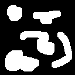
On Linux, you can compile it using:
g++ blob.cpp -o blob -lopencv_core -lopencv_highgui -lopencv_imgproc
The results …

Generating all possible views of a planar object
So it’s Boxing Day and I haven’t got much on, so why not another blog post! yay!
Today’s post is about generating synthetic views of planar objects, such as a book. I needed to do whilst implementing my own version of the Fern algorithm. Here are some references, for your reference …
- M. Ozuysal, M. Calonder, V. Lepetit and P. Fua, Fast Keypoint Recognition using Random Ferns, IEEE Transactions on Pattern Analysis and Machine Intelligence, Vol. 32, Nr. 3, pp. 448 – 461, March 2010.
- M. Ozuysal, P. Fua and V. Lepetit, Fast Keypoint Recognition in Ten Lines of Code, Conference on Computer Vision and Pattern Recognition, Minneapolis, MI, June 2007.
Also check out their website here.
In summary it’s a cool technique for feature matching that is rotation, scale, lighting, and affine viewpoint invariant, much like SIFT, but does it in a simpler way. Fern does this by generating lots of random synthetic views of the planar object and learns (semi-naive Bayes) the features extracted at each view. Because it has seen virtually every view possible, the feature descriptor can be very simple and does not need to be invariant to all the properties mentioned earlier. In fact, the feature descriptor is made up of random binary comparisons. This is in contrast to the more complex SIFT descriptor that has to cater for all sorts of invariance.
I wrote a non-random planar view generator, which is much easier to interpret from a geometric point of view. I find the idea of random affine transformations tricky to interpret, since they’re a combination of translation/rotation/scalings/shearing. My version treats the planar object as a flat piece of paper in 3D space (with z=0), applies a 3×3 rotation matrix (parameterise by yaw/pitch/roll), then re-projects to 2D using an orthographic projection/affine camera (by keeping x,y and ignoring z). I do this process for all combinations of scaling, yaw, pitch, roll I’m interested in.
I use the following settings for Fern
- scaling of 1.0, 0.5, 0.25
- yaw, 0 to 60 degrees, increments of 10 degrees
- pitch, 0 to 60 degrees, increments of 10 degrees
- roll, 0 to 360 degrees, increments of 10 degrees
There’s not much point going beyond 60 degrees for yaw/pitch, you can hardly see the object.
Here are some example outputs


Download
You can download my demo code here SyntheticPlanarView.tar.gz
You will need OpenCV 2.x installed, and compile using the included CodeBlocks project or an IDE of your choice. Run it on the command line with an image as the argument. Hit any key to step through all the view generated.
K-Means for Octave
Googling for K-Means for Octave brought me to this Matlab/Octave script http://www.christianherta.de/kmeans.html by Christian Herta. Works great, except that it ran very slow. Here is my improved version to run faster, most of the expensive for loops have been replaced with faster ones. The new version runs orders of magnitude faster.
function[centroid, pointsInCluster, assignment]= myKmeans(data, nbCluster)
% usage
% function[centroid, pointsInCluster, assignment]=
% myKmeans(data, nbCluster)
%
% Output:
% centroid: matrix in each row are the Coordinates of a centroid
% pointsInCluster: row vector with the nbDatapoints belonging to
% the centroid
% assignment: row Vector with clusterAssignment of the dataRows
%
% Input:
% data in rows
% nbCluster : nb of centroids to determine
%
% (c) by Christian Herta ( www.christianherta.de )
% Modified by Nghia Ho to improve speed

data_dim = length(data(1,:));
nbData   = length(data(:,1));

% init the centroids randomly
data_min = min(data);
data_max = max(data);
data_diff = data_max .- data_min ;

% every row is a centroid
centroid = rand(nbCluster, data_dim);
centroid = centroid .* repmat(data_diff, nbCluster, 1) + repmat(data_min, nbCluster, 1);

% no stopping at start
pos_diff = 1.;

% main loop until

while pos_diff > 0.0
  % E-Step
  assignment = [];

  % assign each datapoint to the closest centroid

  if(nbCluster == 1) % special case
	assignment = ones(size(data,1), 1);
  else
	  dists = [];
	  for c = 1: nbCluster
		d = data - repmat(centroid(c,:), size(data,1), 1);
		d = d .* d;
		d = sum(d, 2); % sum the row values

		dists = [dists d];
	  end

	  [a, assignment] = min(dists');

	  assignment = assignment';
  end

  % for the stoppingCriterion
  oldPositions = centroid;

  % M-Step
  % recalculate the positions of the centroids
  centroid = zeros(nbCluster, data_dim);
  pointsInCluster = zeros(nbCluster, 1);

  for c = 1: nbCluster
	indexes = find(assignment == c);
	d = data(indexes,:);
	centroid(c,:) = sum(d,1);
	pointsInCluster(c,1) = size(d,1);

    if( pointsInCluster(c, 1) != 0)
      centroid( c , : ) = centroid( c, : ) / pointsInCluster(c, 1);
    else
      % set cluster randomly to new position
      centroid( c , : ) = (rand( 1, data_dim) .* data_diff) + data_min;
    end
  end

  %stoppingCriterion
  pos_diff = sum (sum( (centroid .- oldPositions).^2 ) );
end
end
Fast approximate arctan/atan function
While searching for a fast arctan approximation I came across this paper:
“Efficient approximations for the arctangent function”, Rajan, S. Sichun Wang Inkol, R. Joyal, A., May 2006
Unfortunately I no longer have access to the IEEE papers (despite paying for yearly membership, what a joke …), but fortunately the paper appeared in a book that Google has for preview (for selected pages), “Streamlining digital signal processing: a tricks of the trade guidebook”. Even luckier, Google had the important pages on preview. The paper presents 7 different approximation, each with varying degree of accuracy and complexity.
Here is one algorithm I tried, which has a reported maximum error 0.0015 radians (0.085944 degrees), lowest error in the paper.
double FastArcTan(double x)
{
    return M_PI_4*x - x*(fabs(x) - 1)*(0.2447 + 0.0663*fabs(x));
}
The valid range for x is between -1 and 1. Comparing the above with the standard C atan function for 1,000,000 calls using GCC gives:
| Time ms | |
| FastArcTan | 17.315 |
| Standard C atan | 60.708 |
About 3x times faster, pretty good!
OpenCV vs. Armadillo vs. Eigen on Linux revisited
This is a quick revisit to my recent post comparing 3 different libraries with matrix support. As suggested by one of the comments to the last post, I’ve turned off any debugging option that each library may have. In practice you would have them on most of the time for safety reasons, but for this test I thought it would be interesting to see it turned off.
Armadillo and Eigen uses the define ARMA_NO_DEBUG and NDEBUG respectively to turn off error checking. I could not find an immediate way to do the same thing in OpenCV, unless I edit the source code, but chose not to. So keep that in that mind. I also modified the number of iterations for each of the 5 operation performed to be slightly more accurate. Fast operations like add, multiply, transpose and invert have more iterations performed to get a better average, compared to SVD, which is quite slow.
On with the results …
Add
Performing C = A + B
Raw data
| Results in ms | OpenCV | Armadillo | Eigen |
| 4×4 | 0.00093 | 0.00008 | 0.00007 |
| 8×8 | 0.00039 | 0.00006 | 0.00015 |
| 16×16 | 0.00066 | 0.00030 | 0.00059 |
| 32×32 | 0.00139 | 0.00148 | 0.00194 |
| 64×64 | 0.00654 | 0.00619 | 0.00712 |
| 128×128 | 0.02454 | 0.02738 | 0.03225 |
| 256×256 | 0.09144 | 0.11315 | 0.10920 |
| 512×512 | 0.47997 | 0.57668 | 0.47382 |
Normalised
| Speed up over slowest | OpenCV | Armadillo | Eigen |
| 4×4 | 1.00x | 12.12x | 14.35x |
| 8×8 | 1.00x | 6.53x | 2.63x |
| 16×16 | 1.00x | 2.19x | 1.13x |
| 32×32 | 1.39x | 1.31x | 1.00x |
| 64×64 | 1.09x | 1.15x | 1.00x |
| 128×128 | 1.31x | 1.18x | 1.00x |
| 256×256 | 1.24x | 1.00x | 1.04x |
| 512×512 | 1.20x | 1.00x | 1.22x |
Multiply
Performing C = A * B
Raw data
| Results in ms | OpenCV | Armadillo | Eigen |
| 4×4 | 0.00115 | 0.00017 | 0.00086 |
| 8×8 | 0.00195 | 0.00078 | 0.00261 |
| 16×16 | 0.00321 | 0.00261 | 0.00678 |
| 32×32 | 0.01865 | 0.01947 | 0.02130 |
| 64×64 | 0.15366 | 0.33080 | 0.07835 |
| 128×128 | 1.87008 | 1.72719 | 0.35859 |
| 256×256 | 15.76724 | 3.70212 | 2.70168 |
| 512×512 | 119.09382 | 24.08409 | 22.73524 |
Normalised
| Speed up over slowest | OpenCV | Armadillo | Eigen |
| 4×4 | 1.00x | 6.74x | 1.34x |
| 8×8 | 1.34x | 3.34x | 1.00x |
| 16×16 | 2.11x | 2.60x | 1.00x |
| 32×32 | 1.14x | 1.09x | 1.00x |
| 64×64 | 2.15x | 1.00x | 4.22x |
| 128×128 | 1.00x | 1.08x | 5.22x |
| 256×256 | 1.00x | 4.26x | 5.84x |
| 512×512 | 1.00x | 4.94x | 5.24x |
Transpose
Performing C = A^T
Raw data
| Results in ms | OpenCV | Armadillo | Eigen |
| 4×4 | 0.00067 | 0.00004 | 0.00003 |
| 8×8 | 0.00029 | 0.00006 | 0.00008 |
| 16×16 | 0.00034 | 0.00028 | 0.00028 |
| 32×32 | 0.00071 | 0.00068 | 0.00110 |
| 64×64 | 0.00437 | 0.00592 | 0.00500 |
| 128×128 | 0.01552 | 0.06537 | 0.03486 |
| 256×256 | 0.08828 | 0.40813 | 0.20032 |
| 512×512 | 0.52455 | 1.51452 | 0.77584 |
Normalised
| Speed up over slowest | OpenCV | Armadillo | Eigen |
| 4×4 | 1.00x | 17.61x | 26.76x |
| 8×8 | 1.00x | 4.85x | 3.49x |
| 16×16 | 1.00x | 1.20x | 1.21x |
| 32×32 | 1.56x | 1.61x | 1.00x |
| 64×64 | 1.35x | 1.00x | 1.18x |
| 128×128 | 4.21x | 1.00x | 1.88x |
| 256×256 | 4.62x | 1.00x | 2.04x |
| 512×512 | 2.89x | 1.00x | 1.95x |
Inversion
Performing C = A^-1
Raw data
| Results in ms | OpenCV | Armadillo | Eigen |
| 4×4 | 0.00205 | 0.00046 | 0.00271 |
| 8×8 | 0.00220 | 0.00417 | 0.00274 |
| 16×16 | 0.00989 | 0.01255 | 0.01094 |
| 32×32 | 0.06101 | 0.05146 | 0.05023 |
| 64×64 | 0.41286 | 0.25769 | 0.27921 |
| 128×128 | 3.60347 | 3.76052 | 1.88089 |
| 256×256 | 33.72502 | 23.10218 | 11.62692 |
| 512×512 | 285.03784 | 126.70175 | 162.74253 |
Normalised
| Speed up over slowest | OpenCV | Armadillo | Eigen |
| 4×4 | 1.32x | 5.85x | 1.00x |
| 8×8 | 1.90x | 1.00x | 1.52x |
| 16×16 | 1.27x | 1.00x | 1.15x |
| 32×32 | 1.00x | 1.19x | 1.21x |
| 64×64 | 1.00x | 1.60x | 1.48x |
| 128×128 | 1.04x | 1.00x | 2.00x |
| 256×256 | 1.00x | 1.46x | 2.90x |
| 512×512 | 1.00x | 2.25x | 1.75x |
SVD
Performing full SVD, [U,S,V] = SVD(A)
Raw data
| Results in ms | OpenCV | Armadillo | Eigen |
| 4×4 | 0.01220 | 0.22080 | 0.01620 |
| 8×8 | 0.01760 | 0.05760 | 0.03340 |
| 16×16 | 0.10700 | 0.16560 | 0.25540 |
| 32×32 | 0.51480 | 0.70230 | 1.13900 |
| 64×64 | 3.63780 | 3.43520 | 6.63350 |
| 128×128 | 27.04300 | 23.01600 | 64.27500 |
| 256×256 | 240.11000 | 210.70600 | 675.84100 |
| 512×512 | 1727.44000 | 1586.66400 | 6934.32300 |
Normalised
Discussion
Overall, the average running time has decreased for all the operations, which is a good start. Even OpenCV has lower running time, maybe the NDEBUG has an affect, since it’s a standardised define.
| Speed up over slowest | OpenCV | Armadillo | Eigen |
| 4×4 | 18.10x | 1.00x | 13.63x |
| 8×8 | 3.27x | 1.00x | 1.72x |
| 16×16 | 2.39x | 1.54x | 1.00x |
| 32×32 | 2.21x | 1.62x | 1.00x |
| 64×64 | 1.82x | 1.93x | 1.00x |
| 128×128 | 2.38x | 2.79x | 1.00x |
| 256×256 | 2.81x | 3.21x | 1.00x |
| 512×512 | 4.01x | 4.37x | 1.00x |
Discussion
Overall, average running time has decreased for all operations, which is a good sign. Even OpenCV, maybe the NDEBUG has an affect, since it’s a standardised define.
The results from the addition test show all 3 libraries giving more or less the same result. This is probably not a surprise since adding matrix is a very straight forward O(N) task.
The multiply test is a bit more interesting. For matrix 64×64 or larger, there is a noticeable gap between the libraries. Eigen is very fast, with Armadillo coming in second for matrix 256×256 or greater. I’m guessing for larger matrices Eigen and Armadillo leverages the extra CPU core, because I did see all the CPU cores utilised briefly during benchmarking.
The transpose test involve shuffling memory around. This test is affected by the CPU’s caching mechanism. OpenCV does a good job as the matrix size increases.
The inversion test is a bit of a mixed bag. OpenCV seems to be the slowest out of the two.
The SVD test is interesting. Seems like there is a clear range where OpenCV and Armadillo are faster. Eigen lags behind by quite a bit as the matrix size increases.
Conclusion
In practice, if you just want a matrix library and nothing more then Armadillo or Eigen is probably the way to go. If you want something that is very portable with minimal effort then choose Eigen, because the entire library is header based, no library linking required. If you want the fastest matrix code possible then you can be adventurous and try combining the best of each library.
Download
Code compiled with:
g++ test_matrix_lib.cpp -o test_matrix_lib -lopencv_core -larmadillo -lgomp -fopenmp \
-march=native -O3 -DARMA_NO_DEBUG -DNDEBUG
OpenCV vs. Armadillo vs. Eigen on Linux
In this post I’ll be comparing 3 popular C++ matrix libraries found on Linux.
OpenCV is a large computer vision library with matrix support. Armadillo wraps around LAPACK. Eigen is an interesting library, all the implementation is in the C++ header, much like boost. So it is simple to link into, but takes more time compile.
The 5 matrix operations I’ll be focusing on are: add, multiply, transpose, inversion, SVD. These are the most common functions I use. All the libraries are open source and run on a variety of platforms but I’ll just be comparing them on Ubuntu Linux.
Each of the 5 operations were tested on randomly generated matrices of different size NxN with the average running time recorded.
I was tossing up whether to use a bar chart to display the result but the results span over a very large interval. A log graph would show all the data easily but make numerical comparisons harder. So in the end I opted to show the raw data plus a normalised version to compare relative speed ups. Values highlight in red indicate the best results.
Add
Performing C = A + B
Raw data
| Results in ms | OpenCV | Armadillo | Eigen |
| 4×4 | 0.00098 | 0.00003 | 0.00002 |
| 8×8 | 0.00034 | 0.00006 | 0.00017 |
| 16×16 | 0.00048 | 0.00029 | 0.00077 |
| 32×32 | 0.00142 | 0.00208 | 0.00185 |
| 64×64 | 0.00667 | 0.00647 | 0.00688 |
| 128×128 | 0.02190 | 0.02776 | 0.03318 |
| 256×256 | 0.23900 | 0.27900 | 0.30400 |
| 512×512 | 1.04700 | 1.17600 | 1.33900 |
Normalised
| Speed up over slowest | OpenCV | Armadillo | Eigen |
| 4×4 | 1.00x | 30.53x | 44.41x |
| 8×8 | 1.00x | 5.56x | 2.02x |
| 16×16 | 1.62x | 2.66x | 1.00x |
| 32×32 | 1.46x | 1.00x | 1.12x |
| 64×64 | 1.03x | 1.06x | 1.00x |
| 128×128 | 1.52x | 1.20x | 1.00x |
| 256×256 | 1.27x | 1.09x | 1.00x |
| 512×512 | 1.28x | 1.14x | 1.00x |
The average running time for all 3 libraries are very similar so I would say there is no clear winner here. In the 4×4 case where OpenCV is much slower it might be due to overhead in error checking.
Multiply
Performing C = A * B
Raw data
| Results in ms | OpenCV | Armadillo | Eigen |
| 4×4 | 0.00104 | 0.00007 | 0.00030 |
| 8×8 | 0.00070 | 0.00080 | 0.00268 |
| 16×16 | 0.00402 | 0.00271 | 0.00772 |
| 32×32 | 0.02059 | 0.02104 | 0.02527 |
| 64×64 | 0.14835 | 0.18493 | 0.06987 |
| 128×128 | 1.83967 | 1.10590 | 0.60047 |
| 256×256 | 15.54500 | 9.18000 | 2.65200 |
| 512×512 | 133.32800 | 35.43100 | 21.53300 |
Normalised
| Speed up over slowest | OpenCV | Armadillo | Eigen |
| 4×4 | 1.00x | 16.03x | 3.52x |
| 8×8 | 3.84x | 3.35x | 1.00x |
| 16×16 | 1.92x | 2.84x | 1.00x |
| 32×32 | 1.23x | 1.20x | 1.00x |
| 64×64 | 1.25x | 1.00x | 2.65x |
| 128×128 | 1.00x | 1.66x | 3.06x |
| 256×256 | 1.00x | 1.69x | 5.86x |
| 512×512 | 1.00x | 3.76x | 6.19x |
Average running time for all 3 are similar up to 64×64, where Eigen comes out as the clear winner.
Transpose
Performing C = A^T.
Raw data
| Results in ms | OpenCV | Armadillo | Eigen |
| 4×4 | 0.00029 | 0.00002 | 0.00002 |
| 8×8 | 0.00024 | 0.00007 | 0.00009 |
| 16×16 | 0.00034 | 0.00019 | 0.00028 |
| 32×32 | 0.00071 | 0.00088 | 0.00111 |
| 64×64 | 0.00458 | 0.00591 | 0.00573 |
| 128×128 | 0.01636 | 0.13390 | 0.04576 |
| 256×256 | 0.12200 | 0.77400 | 0.32400 |
| 512×512 | 0.68700 | 3.44700 | 1.17600 |
Normalised
| Speed up over slowest | OpenCV | Armadillo | Eigen |
| 4×4 | 1.00x | 17.00x | 12.57x |
| 8×8 | 1.00x | 3.45x | 2.82x |
| 16×16 | 1.00x | 1.81x | 1.20x |
| 32×32 | 1.56x | 1.26x | 1.00x |
| 64×64 | 1.29x | 1.00x | 1.03x |
| 128×128 | 8.18x | 1.00x | 2.93x |
| 256×256 | 6.34x | 1.00x | 2.39x |
| 512×512 | 5.02x | 1.00x | 2.93x |
Comparable running time up to 64×64, after which OpenCV is the winner by quite a bit. Some clever memory manipulation?
Inversion
Performing C = A^-1
Raw data
| Results in ms | OpenCV | Armadillo | Eigen |
| 4×4 | 0.00189 | 0.00018 | 0.00090 |
| 8×8 | 0.00198 | 0.00414 | 0.00271 |
| 16×16 | 0.01118 | 0.01315 | 0.01149 |
| 32×32 | 0.06602 | 0.05445 | 0.05464 |
| 64×64 | 0.42008 | 0.32378 | 0.30324 |
| 128×128 | 3.67776 | 4.52664 | 2.35105 |
| 256×256 | 35.45200 | 16.41900 | 17.12700 |
| 512×512 | 302.33500 | 122.48600 | 97.62200 |
Normalised
| Speed up over slowest | OpenCV | Armadillo | Eigen |
| 4×4 | 1.00x | 10.22x | 2.09x |
| 8×8 | 2.09x | 1.00x | 1.53x |
| 16×16 | 1.18x | 1.00x | 1.15x |
| 32×32 | 1.00x | 1.21x | 1.21x |
| 64×64 | 1.00x | 1.30x | 1.39x |
| 128×128 | 1.23x | 1.00x | 1.93x |
| 256×256 | 1.00x | 2.16x | 2.07x |
| 512×512 | 1.00x | 2.47x | 3.10x |
Some mix results up until 128×128, where Eigen appears to be better choice.
SVD
Performing [U,S,V] = SVD(A)
Raw data
| Results in ms | OpenCV | Armadillo | Eigen |
| 4×4 | 0.00815 | 0.01752 | 0.00544 |
| 8×8 | 0.01498 | 0.05514 | 0.03522 |
| 16×16 | 0.08335 | 0.17098 | 0.21254 |
| 32×32 | 0.53363 | 0.73960 | 1.21068 |
| 64×64 | 3.51651 | 3.37326 | 6.89069 |
| 128×128 | 25.86869 | 24.34282 | 71.48941 |
| 256×256 | 293.54300 | 226.95800 | 722.12400 |
| 512×512 | 1823.72100 | 1595.14500 | 7747.46800 |
Normalised
| Speed up over slowest | OpenCV | Armadillo | Eigen |
| 4×4 | 2.15x | 1.00x | 3.22x |
| 8×8 | 3.68x | 1.00x | 1.57x |
| 16×16 | 2.55x | 1.24x | 1.00x |
| 32×32 | 2.27x | 1.64x | 1.00x |
| 64×64 | 1.96x | 2.04x | 1.00x |
| 128×128 | 2.76x | 2.94x | 1.00x |
| 256×256 | 2.46x | 3.18x | 1.00x |
| 512×512 | 4.25x | 4.86x | 1.00x |
Looks like OpenCV and Armadillo are the winners, depending on the size of the matrix.
Discussion
With mix results left, right and centre it is hard to come to any definite conclusion. The benchmark itself is very simple. I only focused on square matrices of power of two, comparing execution speed, not accuracy, which is important for SVD.
What’s interesting from the benchmark is the clear difference in speed for some of the operations depending on the matrix size. Since the margins can be large it can have a noticeable impact on your application’s running time. It would be pretty cool if there was a matrix library that could switch between different algorithms depending on the size/operation requested, fine tuned to the machine it is running on. Sort of like what Atlas/Blas does.
So which library is faster? I have no idea, try them all for your application and see 🙂
Download
Here is the code used to generate the benchmark: test_matrix_lib.cpp
Compiled with:
g++ test_matrix_lib.cpp -o test_matrix_lib -lopencv_core -larmadillo -lgomp -fopenmp -march=native -O3
Using Maxima to help write compact and fast matrix maths code and more
I’ve recently discovered this cool piece of open source software called Maxima. For those unfamiliar, it is a Computer Algebra System (CAS). You can express maths problem using symbols (as oppose to numerical values only) and apply common maths operations like integration, differentiation, matrix manipulation, finding roots, solving for x, simplification etc. etc. to name a few. In fact, it could probably do most of your calculus homework for you, provided the teacher overlooks the fact that you didn’t show any working step.
Maxima operates on the command line but I tend to use the GUI frontend wxMaxima.
Here’s a programming scenario, you need to do a simple matrix operation, like an inversion of a 3×3 matrix to solve a linear problem. You want it fast but don’t want the hassle of linking to an external library, for whatever reason. Sure, you could do a quick Google and probably find an answer or use it as an excuse to play with Maxima. Here is how to do this in wxMaxima.

M is the 3×3 matrix with each element index by some letter. The output can now be translated directly into C, C++ code or whatever your favourite language is. Notice how the denominator is all the same, so you can improve efficiency by storing it into a variable. You can also check if the denominator is near zero, which would indicate a singular matrix that can’t be inverted.
Eigenvalues of a 3×3 matrix? Sure !

Err okay, maybe not such a great idea.
Need to solve Ax = b? Just re-arrange to x = invert(A)b and you got your answers. You probably only need one IF statement and the rest are maths operation. Not a single FOR loop. How’s that for lean and mean code.
Simple Pano Stitcher
In the past I’ve received emails from people on the OpenCV Yahoo group asking for help on panoramic stitching, to which I answered them to the best of my knowledge, though the answers were theoretical. Being the practical man I like to think of myself, I decided to finally get down and dirty and write a simple panoramic stitcher that should help beginners venturing into panoramic stitching. In the process of doing so I learned some new things along the way. I believe OpenCV is scheduled to include some sort of panoramic stitching engine in future release. In the meantime you can check out my Simple Pano Stitcher program here:
Last update: 31/03/2014
Download SimplePanoStitcher-0.2.0.zip
It uses OpenCV to do fundamental image processing stuff and includes a public domain Levenberg-Marquardt non-linear solver.
To compile the code just type make and run bin/Release/SimplePanoStitcher. It will output a bunch of layer-xxx.png images as output. I’ve included sample images in the sample directory, which the program uses by default. Edit the source code to load your own images. You’ll need to know the focal length in pixels used to capture each image.
To keep things simple I only wrote the bare minimum to get it up and running, for more information check the comments in main.cpp at the top of the file.
Results with Simple Pano Stitcher
Below is a sample result I got after combining all the layers, by simply pasting them on top of each other. No fancy blending or anything. On close inspection there is some noticeable parallax. If I had taken it on a tripod instead of hand held it should be less noticeable.

Discussion
One of the crucial steps to getting good results is the non-linear optimisation step. I decided to optimise the focal length, yaw, pitch, and roll for each image. A total of 4 parameters. I thought it would be interesting to compare results with and without any optimisation. For comparison I’ll be using the full size images (3872 x 2592), which is not included in the sample directory to keep the package size reasonable. Below shows a close up section of the roof of the house without optimisation.

The root mean squared error reported is 22.5008 pixels. The results are without a doubt awful! Looking at it too long would cause me to require new glasses with a stronger optical prescription. I’ll now turn on the non-linear optimisation step for the 4 parameters mentioned previously. Below is what we get.

The reported root mean squared error is 3.84413 pixels. Much better! Not perfect, but much more pleasant to look at than the previous image.
There is no doubt a vast improvement by introducing non-linear optimisation to panoramic stitching. One can improve the results further by taking into consideration for radial distortion, but I’ll leave that as an exercise to the reader.
I originally got the focal length for my camera lens from calibration using the sample program (calibration.cpp) in the OpenCV 2.x directory. It performs a standard calibration using a checkerboard pattern. Yet even then its accuracy is still a bit off. This got me thinking a bit. Can we use panoramic stitching to refine the focal length? What are the pros and cons? The images used in the stitching process should ideally be scenery with features that are very very far, so that parallax is not an issue, such as outdoor landscape of mountains or something. Seems obvious enough, there are probably papers out there but I’m too lazy to check at this moment …
KD-tree on GPU for 3D point searching
This post is a follow up on my previous post about using the GPU for brute force nearest neighbour searching. In the previous post I found the GPU to be slower than using the ANN library, which utilises some sort of KD-tree to speed up searches. So I decided to get around to implementing a basic KD-tree on the GPU for a better comparison.
My approach was to build the tree on the host and transfer it to the GPU. Sounds conceptually easy enough, as most things do. The tricky part was transferring the tree structure. I ended up representing the tree as an array node on the GPU, with each node referencing other nodes using an integer index, rather than using pointers, which I suspect would have got rather ugly. The KD-tree that I coded allows the user to set the maximum depth if they want to, which turned out to have some interesting effects as shown shortly. But first lets see some numbers:
nghia@nghia-laptop:~/Projects/CUDA_KDtree$ bin/Release/CUDA_KDtree
CUDA blocks/threads: 196 512
Points in the tree: 100000
Query points: 100000

Results are the same!

GPU max tree depth: 99
GPU create + search: 321.849 + 177.968 = 499.817 ms
ANN create + search: 162.14 + 456.032 = 618.172 ms
Speed up of GPU over CPU for searches: 2.56x
Alright, now we’re seeing better results from the GPU. As you can see I broken the timing down for the create/search part of the KD-tree. My KD-tree creation code is slower than ANN, no real surprise there. However the searches using the GPU is faster, the results I was hoping for. But only 2.56x faster, nothing really to rave about. I could probably get the same speed up, or more, by multi-threading the searches on the CPU. I then started to play around with the maximum depth of my tree and got these results:
GPU max tree depth: 13
GPU create + search: 201.771 + 56.178 = 257.949 ms
ANN create + search: 163.414 + 403.978 = 567.392 ms
Speed up of GPU over CPU for searches: 7.19x
From 2.56x to 7.19x, a bit better! A max tree depth of 13 produced the fastest results. It would seem that there is a sweet spot between creating a tree with the maximum depth required, so that each leaf of the tree holds only a single point, versus a tree with a limited depth and doing a linear search on the leaves. I suspect most of the bottleneck is due to the heavy use of global memory, especially randomly accessing them from different threads, which is why we’re not seeing spectacular speed ups.
The code for the CUDA KD-tree can be downloaded here CUDA_KDtree.zip. Its written for Linux and requires the ANN library to be installed.
Brute Force Nearest Neighbour in CUDA for 3D points
It has been a while since I touched CUDA and seeing as I haven’t posted anything interesting on the front page yet I decided to write a simple brute force nearest neighbour to pass time. The idea has been implemented by the fast kNN library. The library is restricted to non-commerical purposes.
In the past I’ve needed to do nearest neighbour search mainly in 3D space, particular for the Iterative Closest Point (ICP) algorithm, or the likes of it. I relied on the ANN library to do fast nearest neighbour searches, which it does very well. A brute force implementation at the time would have been unimaginably slow and simply impractical. It would have been as slow as watching paint dry for the kind of 3D data I worked on. On second thoughts, watching paint dry would have been faster. Brute force has a typical running time of O(NM), where N and M are the size of the two data set to be compared, basically quadratic running time if both data sets are similar in size. This is generally very slow and impractical for very large data set using the CPU. You would almost be crazy to do so. But on the GPU it is a different story.
I ran a test case where I have 100,000 3D points and 100,000 query points. Each query point searches for its nearest point. This equates to 100,000,000,000 comparisons (that’s a lot of zeros, did I count them right? yep I did). This is what I got on my Intel i7 laptop with a GeForce GTS 360M:
nghia@nghia-laptop:~/Projects/CUDA_NN$ bin/Release/CUDA_NN
Data dimension: 3
Total data points: 100000
Total query points: 100000

GPU: 2193.72 ms
CPU brute force: 69668.3 ms
libANN: 540.008 ms

Speed up over CPU brute force from using GPU: 31.76x
Speed up over libANN using GPU: 0.25x
ANN produces the fastest results for 3D point searching. The GPU brute force version is slower but still practical for real applications, especially given its ease of implementation and reasonable running time.
I’d imagine even greater speed up (orders of magnitude?) is achievable with a KD-tree created on the GPU. A paper describing building a KD-tree on the GPU can be found at http://www.kunzhou.net/. However I could not find any source code on the website. I might give it a shot when I have time.
The demo code I wrote only searches for the nearest point given a query point. Extending the program to find the K nearest neighbour for a bunch of query points should not be too difficult. Each query point would have to maintain a sorted array of indexes and distances.
My code can be downloaded here (CUDA_LK.zip). If you’re on Linux just type make and run CUDA_NN. Just a warning, on Linux if a CUDA program runs for more than 5 second or so the operating system will kill it and display some warning.