Last Updated on February 13, 2013 by nghiaho12
I’ve been fascinated for the past months or so on using RBM (restricted Boltzmann machine) to automatically learn visual features, as oppose to hand crafting them. Alex Krizhevsky’s master thesis, Learning Multiple Layers of Features from Tiny Images, is a good source on this topic. I’ve been attempting to replicate the results on a much smaller set of data with mix results. However, as a by product of I did manage generate some interesting results.
One of the tunable parameters of an RBM (neural network as well) is a weight decay penalty. This regularisation penalises large weight coefficients to avoid over-fitting (used conjunction with a validation set). Two commonly used penalties are L1 and L2, expressed as follows:
where theta is the coefficents of the weight matrix.
L1 penalises the absolute value and L2 the squared value. L1 will generally push a lot of the weights to be exactly zero while allowing some to grow large. L2 on the other hand tends to drive all the weights to smaller values.
Experiment
To see the effect of the two penalties I’ll be using a single RBM with the following configuration:
- 5000 input images, normalized to
- no. of visible units (linear) = 64 (16×16 greyscale images from the CIFAR the database)
- no. of hidden units (sigmoid) = 100
- batch training size = 100
- iterations = 1000
- momentum = 0.9
- learning rate = 0.01
- weight refinement using an autoencoder with 500 iterations and learning rate of 0.01
The weight refinement step uses a 64-100-64 autoencoder with standard backpropagation.
Results
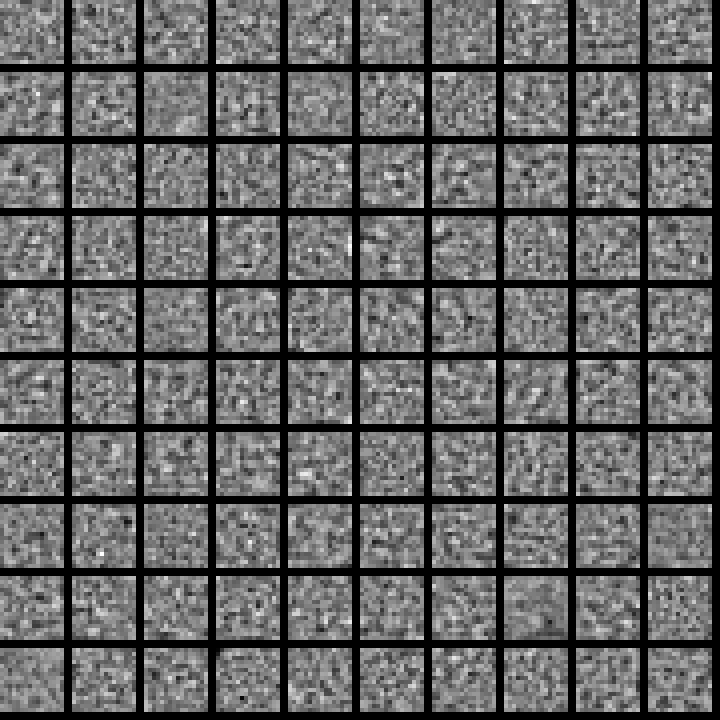
For reference, here are the 100 hidden layer patterns without any weight decay applied:
 As you can see they’re pretty random and meaningless There’s no obvious structure. Though what is amazing is that even with such random patterns you can reconstruct the original 5000 input images quite well using a weighted linear combinations of them.
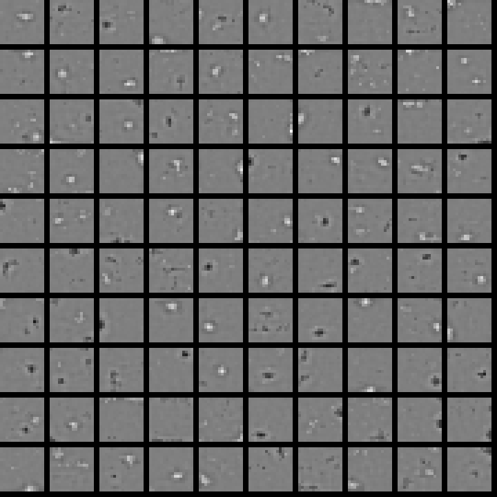
Now applying an L1 weight decay with a weight decay multiplier of 0.01 (which gets multiplied with the learning rate) we get something more interesting:
 We get stronger localised “spot” like features.
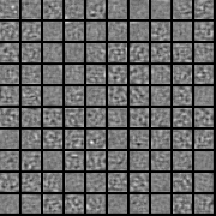
And lastly, applying L2 weight decay with a multiplier of 0.1 we get
 which again looks like a bunch of random patterns except smoother. This has the effect of smoothing the reconstruction image.
Despite some interesting looking patterns I haven’t really observed the edge or Gabor like patterns reported in the literature. Maybe my training data is too small? Need to spend some more time …
You can’t get the Gabor/edge patterns without training a covariance layer like in the threeway mocap demo or Ranzato’s Mean-Covariance beastie. The patterns get made at the covariance layer after you train translation & rotation pairs of random pixel images.
Your first set of features looks like it’s still “confused” to me– it still has a lot of the random initialization jaggies which haven’t gotten smoothed out yet. Decay will smoothen it, more epochs will too.
What does your reconstruction error curve look like?
I got pretty decent results after training it on much smaller patches eg. 5×5, which I didn’t bother posting up. The bigger patches are much harder to extract meaningful features. I’ve seen the same behaviour with a convolutional neural network as well.
I didn’t record the reconstruction error curve but that’s definitely a good idea.
I find doing better on bigger patches needs better selectivity/sparsity than the vanilla RBM. Ranzato does this by setting his hidden bias to -1 initially (instead of 0). A different dude did it with -4. But this is major weaksauce compared to Goh’s sparsity/selectivity regularizer (which can make RBMs do a lot of cool things by tweaking the extra hyper parameters).
I like Goh’s idea very much, blend in an ideal set of hiddens with the training data’s hiddens because it allows for very different optimizations including neural network/emotional driven ideals!
Actually, experimenting with Ranzato’s works, it’s actually NOT the covariance layer nor the feature**2 step that causes the Gaborness.
What causes the Gabor filters is the initialization of the feature weights. If you initialize them with small random values (like “normal”), you get bumpy/staticky/uninteresting features. But Ranzato initializes his hidden layer (that sits on the covar layer) to numpy.eye, ie the Identity matrix. Trying this on a plain on RBM on MNIST and I get the “pen strokes” after multiplying the identity matrix by .5!
This sounds interesting, I’ll have to be check out Ranzato’s work.
Hi, I’ve been wanting to implement an L1 Regularization on an RBM but have not yet understood how to implement it. How do you implement yours?
regards,
Lintang
Have a look at the code, it’s been a while so I don’t remember it well.
Hi Where is the code?
http://nghiaho.com/uploads/code/RBM_Features-0.1.0.tar.gz