Arduino Uno R3 + MaxSonar EZ3 calibration

I recently got my Arduino Uno R3 board this week and simply love how easy it is to use! My first muck around project was using a MaxSonar EZ3 sonar sensor to display the range readings to a serial LED segment display.

The MaxSonar’s output of (Vcc/512) per inch was not as accurate as I’d like it to be. I assumed Vcc = 5V. I decided to calibrate it by taking a few readings using a tape measure and reading the raw readings from the 10bit analog pin, hoping to fit a straight line. Plotting this data gave the following graph
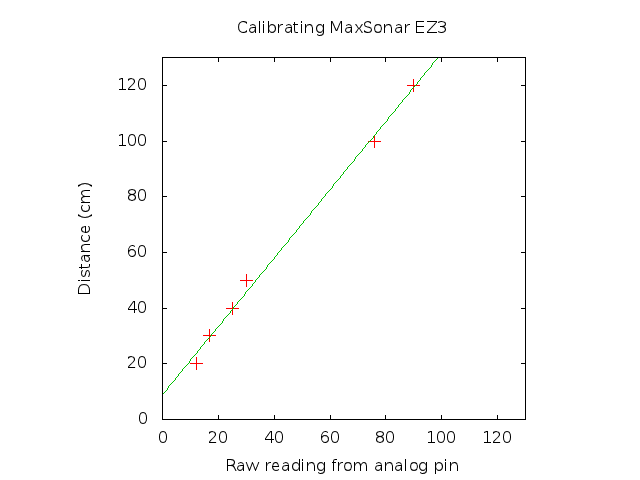
As I hoped it’s a nice linear relationship. I’ve only collected data up to 120cm, ideally you would do it up to the range you’re interested in working to. Fitting a y = mx + c line gave the following values

m = 1.2275

c = 8.8524

So now I have a nice formula for converting the analog reading to range in centimetres. In practice I use fixed point integer maths.

centimetres = 1.2275*analog_reading + 8.8524

The full sketch up code is

void setup()
{
  Serial.begin(9600); 
}

int init_loop = 0;

void loop()
{  
  // NOTE to myself: Arduino Uno int is 16 bit
  const int sonarPin = A0;

  int dist = analogRead(sonarPin);

  // linear equation relating distance vs analog reading
  // y = mx + c
  // m = 1.2275
  // c = 8.8524

  // fixed precision scaling by 100
  dist = dist*123 + 885;
  dist /= 100;

  // output the numbers
  int thousands = dist / 1000;
  int hundreds = (dist - thousands*1000)/100;
  int tens = (dist - thousands*1000 - hundreds*100)/10;
  int ones = dist - thousands*1000 - hundreds*100 - tens*10;

  // Do a few times to make sure the segment display recieves the data ...
  if(init_loop < 5) {
    // Clear the dots
    Serial.print(0x77);
    Serial.print(0x00);

    // Set brightness
    Serial.print("z");
    Serial.print(0x00); // maximum brightness

     init_loop++;
  }

  // reset position, needed in case the serial transmission stuffs up
  Serial.print("v");

  // if thousand digit is zero don't display anything
  if(thousands == 0) {
    Serial.print("x"); // blank
  }
  else {
    Serial.print(thousands);  
  }

  // if thousand digit and hundred digit are zero don't display anything
  if(thousands == 0 && hundreds == 0) {
    Serial.print("x");
  }
  else {
    Serial.print(hundreds);  
  }

  // always display the tens and ones
  Serial.print(tens);  
  Serial.print(ones);

  delay(100);
}

To get the raw analog reading comment out the bit where it calculates the distance using the linear equation.

Below is a picture of the hardware setup. The MaxSonar is pointing up the ceiling, which I measured with a tape measure to be about 219 cm. The readout from the Arduino is 216cm, so it’s not bad despite calibrating up to 120cm only.

Quirks and issues

It took me a while to realise an int is 16bit on the Arduino! (fail …) I was banging my head wondering why some simple integer maths was failing. I have to be conscious of my scaling factors when doing fixed point maths.

After compiling and uploading code to the Arduino I found myself having to unplug and plug it back in for the serial LED segment display to function correctly. It seems to leave it in an unusable state during the uploading process.

Multivariate decision tree (decision tree + linear classifier)

I’ve been mucking around with a multivariate decision tree for the past few days in Octave. Mostly out of curiosity. It’s basically a decision tree that uses a hyper plane to split the data at each node, instead of splitting at a single attribute. For example, say we have 2D data (x,y), a node in a standard decision tree might look like

if x > 5

where as a multivariate might be

if \theta_{1}x + \theta_{2}y + \theta_{3} > 0

The idea seems to have been around since the early 90s but for some reason you don’t hear about them nowadays. Maybe for good reason? Either way still an interesting idea. My implementation uses RANSAC to find a good hyper plane to split the data and uses the ‘Information Gain’/Entropy formula  to measure the “goodness” of the hyper plane.

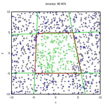
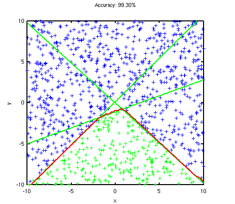
Below are two simple synthetic test data that a decision tree and linear classifier might have trouble with, but when combined together they perform quite well. The green lines are the individual linear decision boundaries at each node and the red is the final boundary. The green samples are labelled “positive” and blue is “negative”. The accuracy of the classification is shown in the title of the graph.


The first dataset above cannot be separated using a single linear decision boundary, where as a decision tree on the other hand will probably zig-zag along the diagonal boundary producing a bigger tree than necessary. The multivariate decision tree on the other hand separates the data in 3 cuts. It is close to what I would consider the best, which would be 2 cuts along the diagonal boundaries. This is interesting, because it seems to suggest that to get the best decision boundary a sub-optimal cut might be required at some stage! I wonder if there’s a way to re-visit the boundary lines and simplify them …

The second dataset consists of positive samples shaped in a circle enclosed by negative samples. Pretty typical synthetic dataset. Again, no single linear decision boundary will separate this. But a decision tree will probably produce similar result to what I got given only 4 cuts as well.

Download

Download the Octave script. Might need to do right click save as.

MultivariateDecisionTree.7z

Extract and call Run.m, that’s capital R and not ‘run’ !

Rotation invariance using Harris corners

This post on how to take advantage of the Harris corner to calculate dominant orientations for a feature patch, thus achieving rotation invariance. Some popular examples are the SIFT/SURF descriptors. I’ll present an alternative way that is simple to implement, especially if you’re already using Harris corners.

Background

The Harris corner detector is an old school feature detector that is still used today. Given an NxN pixel patch, and the horizontal/vertical derivatives extracted from it (via Sobel for example), it accumulates the following matrix

A = \frac{1}{N^2} \left[\begin{array}{cc} I_{x}^2 & I_{x}I_{y} \\ I_{x}I_{y} & I_{y}^2 \end{array} \right]

where

I_{x} is the summation of the derivatives in the x direction and I_{y} in the y direction for every pixel. The \frac{1}{N^2} averages the summation. Mathematically you don’t really need to do this, but in practice due to numerical overflow you want to keep the values in the matrix reasonably small. The 2×2 matrix above is the result of doing the following operation

Let B = \left[\begin{array}{cc} ix_{1} & iy_{1} \\ ix_{2} & iy_{2} \\ . & . \\ . & . \\ ix_{n} & iy_{n} \end{array} \right]

where ix_{n} and iy_{n} are the derivatives at pixel n.

Using B we get

A = B^{T}B

You can think of matrix A as the covariance matrix, and the values in B are assumed to be centred around zero.

Once the matrix A is calculated there are a handful of ways to calculate the corner response of the patch, which I won’t be discussing here.

Rotation invariance

With the matrix A, the orientation of the patch can be calculated using the fact that the eigenvectors of A can be directly converted to a rotation angle as follows (note: matrix are index as A(row,col) )

t = trace(A) = A(1,1) + A(2,2)

d = determinant(A) = A(1,1)*A(2,2) - A(1,2)*A(2,1)

eig1 = t/2 + \sqrt{t^{2}/4 - d}

angle = atan2\left(A(2,1), eig1 - A(2,2)\right)

eig1 is the larger of the two eigenvalues, which corresponds to the eigenvector

v = \left[\begin{array}{c} eig1 - d \\ A(2,1) \end{array} \right]

The eigenvalue/eigenvector was calculated using an algebraic formula I found here.

I’ve found in practice that the above equation results in an uncertainty in the angle, giving two possibilities

angle1 = angle

angle2 = angle + 180 degrees

I believe this is because an eigenvector can point in two directions, both of which are correct. If v is an eigenvector then -v is legit as well. A negation means a 180 degree rotation. So there are in fact two dominant orientations for the patch. So how do we resolve this? We don’t, keep them both!

Example

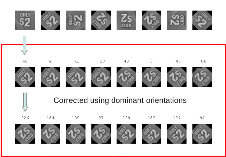
Here’s an example of a small 64×64 patch rotated from 0 to 360, every 45 degrees. The top row is the rotated patch, the second row is the rotation corrected patch using angle1 and the third row using angle2. The numbers at the top of the second/third rows are the angles in degrees of the rotated patches. You can see there are in fact only two possible appearances for the patch after it has been rotated using the dominant orientation.

Interestingly, the orientation angles seem to have a small error. For example, compare patch 1 and patch 5 (counting from the left). Patch 1 and patch 5 differ by 180 degrees, yet the orientations are 46 and 49 degrees respectively, a 3 degree difference. I think this might be due to the bilinear interpolation when I was using the imrotate function in Octave. I’ve tried using an odd size patch eg. 63×63, thinking it might be a centring issue when rotating but still the same results. For now it’s not such a big deal.

Rotation invariance using Harris corners

Implementation notes

I used a standard 3×3 Sobel filter to get the pixel derivatives. When accumulating the A matrix, I only use pixels within the largest circle (radius 32) enclosed by the 64×64 patch, instead of all pixels. This makes the orientation more accurate, since the corners sometime appear off the image when they are rotated.

Code

Here is the Octave script and image patch used to generate the image above (minus the annotation). Right click and save as to download.

rotation_invariance.m

patch.png

Approximating a Gaussian using a box filter

I came across this topic while searching for a fast Gaussian implementation. It’s approximating a Gaussian by using multiple box filters. It’s old stuff but cool nonetheless. I couldn’t find a reference showing it in action visually that I liked so I decided to whip one up quickly.

The idea is pretty simple, blur the image multiple times using a box filter and it will approximate a Gaussian blur. The box filter convolution mask in 1D looks something like [1 1 1 1] * 0.25 , depending how large you want the blurring mask to be. Basically it just calculates the average value inside the mask.

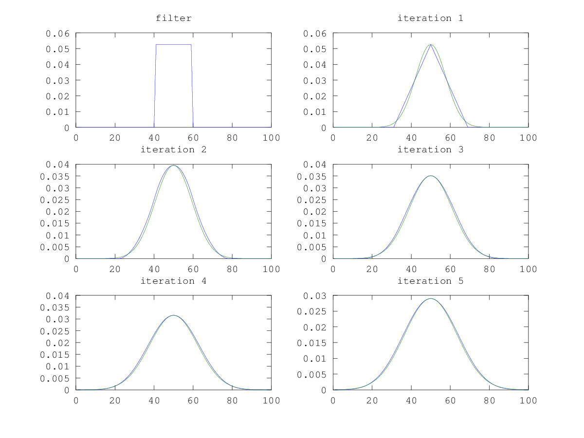
Alright enough yip yapping, lets see it in action! Below shows 6 graphs. The first one labelled ‘filter’ is the box filter used. It is a box 19 units wide, with height 1/19. Subsequent graphs are the result of recursively convolving the box filter with itself. The blue graph is the result of the convolution, while the green is the best Gaussian fit for the data.

Gaussian approximation using box filter

After the 1st iteration the plot starts to look like a Gaussian very quickly. This link from Wikipedia says 3 iterations will approximate a Gaussian to within roughly 3%. It also gives a nice rule of thumb for calculating the length of the box based on the desired standard deviation.

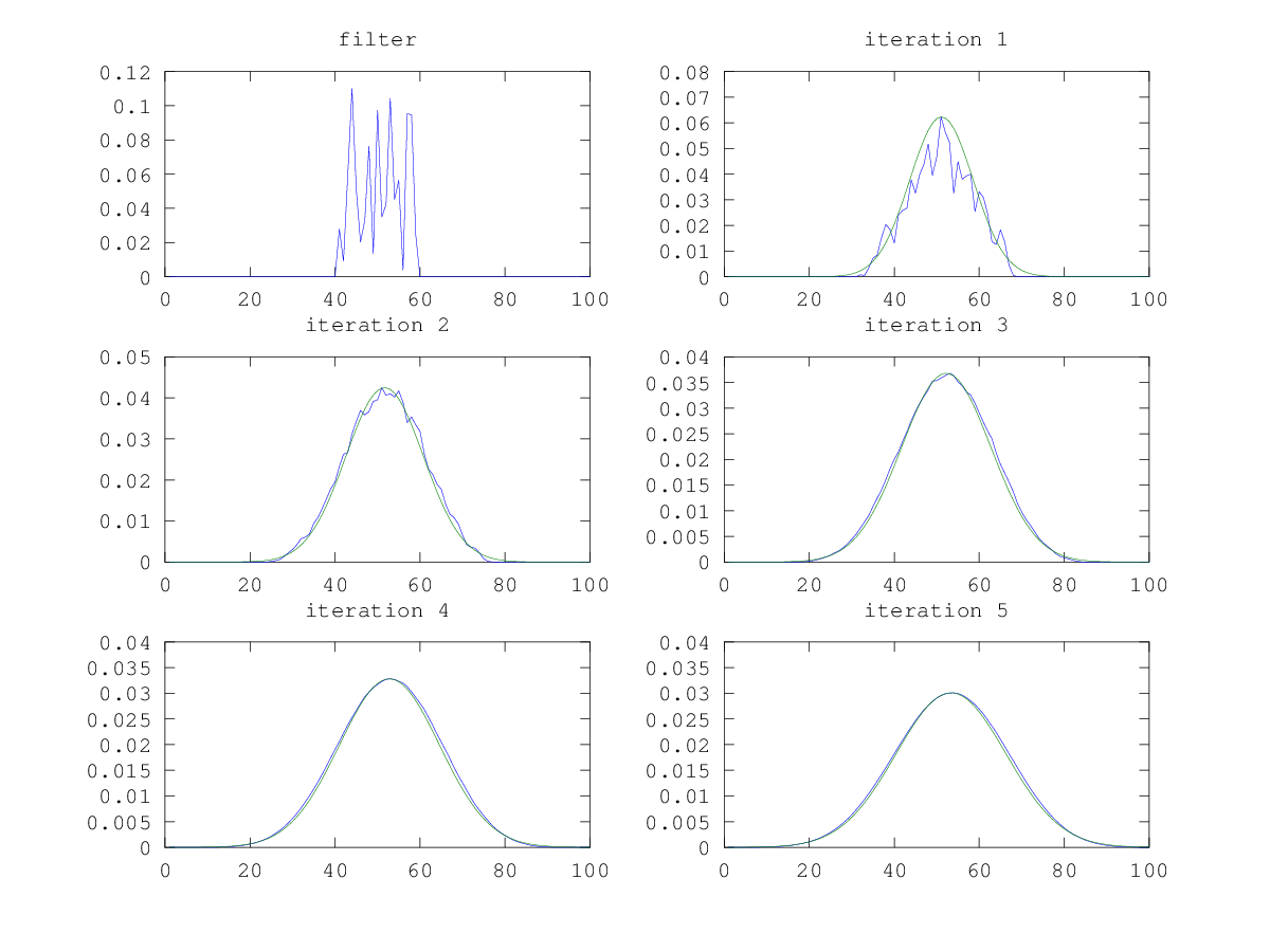
What’s even cooler is that this works with ANY filter, provided all the values are positive! The graph below shows convolving with a filter made up of random positive values.

Gaussian approximation using a random filter

The graph starts to smooth out after the 3rd iteration.

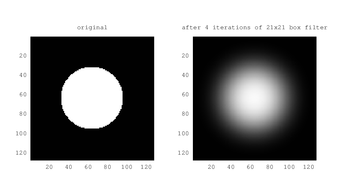
Another example, but with an image instead of a 1D signal.

For the theory behind why this all works have a search for the Central Limit Theorem. The Wikipedia article is a horrible read if you’re not a maths geek. Instead, I recommend watching this Khan Academy video instead to get a good idea.

The advantage of the box filter is that it can be implemented very efficiently for 2D blurring by first separating the mask into 1D horizontal/vertical mask and re-using calculated values. This post on Stackoverflow has a good discussion on the topic.

Code

You can download my Octave script to replicate the results above or fiddle around with. Download by right clicking and saving the file.

box_demo.m
box_demo2.m

Quick and easy connected component (blob) using OpenCV

UPDATE: June 2015

Check the link below to see if it meets your need first.

http://docs.opencv.org/3.0-beta/modules/imgproc/doc/structural_analysis_and_shape_descriptors.html?highlight=connectedcomponents#connectedcomponents


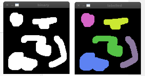
OpenCV is up to version 2.3.1 and it still lacks a basic connected component function for binary blob analysis. A quick Google will bring up cvBlobsLib (http://opencv.willowgarage.com/wiki/cvBlobsLib), an external lib that uses OpenCV calls. At the time when I needed such functionality I wasn’t too keen on linking to more libraries for something so basic. So instead I quickly wrote my own version using existing OpenCV calls. It uses cv:floodFill with 4 connected neighbours. Here is the code and example input image

UPDATE: 22th July 2013

I got rid of the hacks to work with OpenCV 2.3.1. It should now work with OpenCV 2.4.x.

On Linux, you can compile it using:

g++ blob.cpp -o blob -lopencv_core -lopencv_highgui -lopencv_imgproc

The results …

Generating all possible views of a planar object

So it’s Boxing Day and I haven’t got much on, so why not another blog post! yay!

Today’s post is about generating synthetic views of planar objects, such as a book. I needed to do whilst implementing my own version of the Fern algorithm. Here are some references, for your reference …

  • M. Ozuysal, M. Calonder, V. Lepetit and P. Fua, Fast Keypoint Recognition using Random Ferns, IEEE Transactions on Pattern Analysis and Machine Intelligence, Vol. 32, Nr. 3, pp. 448 – 461, March 2010.
  • M. Ozuysal, P. Fua and V. Lepetit, Fast Keypoint Recognition in Ten Lines of Code, Conference on Computer Vision and Pattern Recognition, Minneapolis, MI, June 2007.

Also check out their website here.

In summary it’s a cool technique for feature matching that is rotation, scale, lighting, and affine viewpoint invariant, much like SIFT, but does it in a simpler way. Fern does this by generating lots of random synthetic views of the planar object and learns (semi-naive Bayes) the features extracted at each view. Because it has seen virtually every view possible, the feature descriptor can be very simple and does not need to be invariant to all the properties mentioned earlier. In fact, the feature descriptor is made up of random binary comparisons. This is in contrast to the more complex SIFT descriptor that has to cater for all sorts of invariance.

I wrote a non-random planar view generator, which is much easier to interpret from a geometric point of view. I find the idea of random affine transformations tricky to interpret, since they’re a combination of translation/rotation/scalings/shearing. My version treats the planar object as a flat piece of paper in 3D space (with z=0), applies a 3×3 rotation matrix (parameterise by yaw/pitch/roll), then re-projects to 2D using an orthographic projection/affine camera (by keeping x,y and ignoring z). I do this process for all combinations of scaling, yaw, pitch, roll I’m interested in.

I use the following settings for Fern

  • scaling of 1.0, 0.5, 0.25
  • yaw, 0 to 60 degrees, increments of 10 degrees
  • pitch, 0 to 60 degrees, increments of 10 degrees
  • roll, 0 to 360 degrees, increments of 10 degrees

There’s not much point going beyond 60 degrees for yaw/pitch, you can hardly see the object.

Here are some example outputs

Download

You can download my demo code here SyntheticPlanarView.tar.gz

You will need OpenCV 2.x installed, and compile using the included CodeBlocks project or an IDE of your choice. Run it on the command line with an image as the argument. Hit any key to step through all the view generated.

K-Means for Octave

Googling for K-Means for Octave brought me to this Matlab/Octave script http://www.christianherta.de/kmeans.html by Christian Herta. Works great, except that it ran very slow. Here is my improved version to run faster, most of the expensive for loops have been replaced with faster ones. The new version runs orders of magnitude faster.

 
function[centroid, pointsInCluster, assignment]= myKmeans(data, nbCluster)
% usage
% function[centroid, pointsInCluster, assignment]=
% myKmeans(data, nbCluster)
%
% Output:
% centroid: matrix in each row are the Coordinates of a centroid
% pointsInCluster: row vector with the nbDatapoints belonging to
% the centroid
% assignment: row Vector with clusterAssignment of the dataRows
%
% Input:
% data in rows
% nbCluster : nb of centroids to determine
%
% (c) by Christian Herta ( www.christianherta.de )
% Modified by Nghia Ho to improve speed

data_dim = length(data(1,:));
nbData   = length(data(:,1));

% init the centroids randomly
data_min = min(data);
data_max = max(data);
data_diff = data_max .- data_min ;

% every row is a centroid
centroid = rand(nbCluster, data_dim);
centroid = centroid .* repmat(data_diff, nbCluster, 1) + repmat(data_min, nbCluster, 1);

% no stopping at start
pos_diff = 1.;

% main loop until

while pos_diff > 0.0
  % E-Step
  assignment = [];

  % assign each datapoint to the closest centroid

  if(nbCluster == 1) % special case
	assignment = ones(size(data,1), 1);
  else
	  dists = [];
	  for c = 1: nbCluster
		d = data - repmat(centroid(c,:), size(data,1), 1);
		d = d .* d;
		d = sum(d, 2); % sum the row values

		dists = [dists d];
	  end

	  [a, assignment] = min(dists');

	  assignment = assignment';
  end

  % for the stoppingCriterion
  oldPositions = centroid;

  % M-Step
  % recalculate the positions of the centroids
  centroid = zeros(nbCluster, data_dim);
  pointsInCluster = zeros(nbCluster, 1);

  for c = 1: nbCluster
	indexes = find(assignment == c);
	d = data(indexes,:);
	centroid(c,:) = sum(d,1);
	pointsInCluster(c,1) = size(d,1);

    if( pointsInCluster(c, 1) != 0)
      centroid( c , : ) = centroid( c, : ) / pointsInCluster(c, 1);
    else
      % set cluster randomly to new position
      centroid( c , : ) = (rand( 1, data_dim) .* data_diff) + data_min;
    end
  end

  %stoppingCriterion
  pos_diff = sum (sum( (centroid .- oldPositions).^2 ) );
end
end

Fast approximate arctan/atan function

While searching for a fast arctan approximation I came across this paper:

Efficient approximations for the arctangent function”, Rajan, S. Sichun Wang Inkol, R. Joyal, A., May 2006

Unfortunately I no longer have access to the IEEE papers (despite paying for yearly membership, what a joke …), but fortunately the paper appeared in a book that Google has for preview (for selected pages), “Streamlining digital signal processing: a tricks of the trade guidebook”. Even luckier, Google had the important pages on preview. The paper presents 7 different approximation, each with varying degree of accuracy and complexity.

Here is one algorithm I tried, which has a reported maximum error 0.0015 radians (0.085944 degrees), lowest error in the paper.

double FastArcTan(double x)
{
    return M_PI_4*x - x*(fabs(x) - 1)*(0.2447 + 0.0663*fabs(x));
}

The valid range for x is between -1 and 1. Comparing the above with the standard C atan function for 1,000,000 calls using GCC gives:

Time ms
FastArcTan 17.315
Standard C atan 60.708

About 3x times faster, pretty good!

Automatic doctoral advisor genealogy diagram using Wikipedia

An idea to me occured some time ago when I was bored and browsing through Wikipedia looking up famous historical figures in science. At the time, I was interested in each person’s supervisor and kept clicking the doctoral advisor link in their bio box to see where it would take me. Some went as far back as the 17th century. I thought it would be a nifty idea to hack togther a quick script that would grab data from Wikipedia and automatically output a tree diagram showing the PhD genealogy/lineage. So I did it.

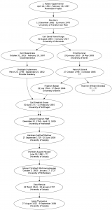
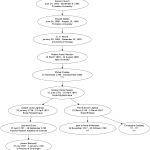
Here are the results for two people I chose. The first is Alan Turing (aka the father of computer science) and the second is Robert Oppenheimer (aka the father of the atomic bomb). I have a thing for a World War 2 scientists.

The arrow points to the doctoral advisor of the current node. Alan Turing’s doctoral lineage has some very well known names that I’ve come across during my studies in engineering;  Bernoulli, Poisson, Euler, Laplace and Lagrange. Wow, that’s a lot! There’s also Gauss that appears on Robert Oppenheimer’s side.

Robert Oppenheimer

Alan Turing

I’ll probably add more in the upcoming days if I find anything else interesting.

Download

Download doctoral_advisor_tree.zip

The script has been written for Linux and requires PHP and GraphViz installed, both are in Ubuntu’s synaptics. Also, set the file permission of the script to be executable. It’s usage is as follows:

./doctoral_advisor_tree [wiki link] [graph.txt] [graph.png]

wiki link is the actual URL to the Wikipedia page of the person you are interested in, graph.txt is a temporary file created for input into GraphViz. Here’s an example usage:

./doctoral_advisor_tree http://en.wikipedia.org/wiki/John_Forbes_Nash,_Jr. \ 
graph.txt graph.png

You can actually try the above command. It’s for the mathematician John Nash, who gained mainstream popularity from the film based on him, ‘A Beautiful Mind’.

Important

This script is very simple and has not been tested thorughly. It was written in like 2-3 hours. It relies on the Wikipedia page to follow a specific formatting style.

OpenCV vs. Armadillo vs. Eigen on Linux revisited

This is a quick revisit to my recent post comparing 3 different libraries with matrix support. As suggested by one of the comments to the last post, I’ve turned off any debugging option that each library may have. In practice you would have them on most of the time for safety reasons, but for this test I thought it would be interesting to see it turned off.

Armadillo and Eigen uses the define ARMA_NO_DEBUG and NDEBUG respectively to turn off error checking. I could not find an immediate way to do the same thing in OpenCV, unless I  edit the source code, but chose not to. So keep that in that mind. I also modified the number of iterations for each of the 5 operation performed to be slightly more accurate. Fast operations like add, multiply, transpose and invert have more iterations performed to get a better average, compared to SVD, which is quite slow.

On with the results …

Add

Performing C = A + B

Raw data

Results in ms OpenCV Armadillo Eigen
4×4 0.00093 0.00008 0.00007
8×8 0.00039 0.00006 0.00015
16×16 0.00066 0.00030 0.00059
32×32 0.00139 0.00148 0.00194
64×64 0.00654 0.00619 0.00712
128×128 0.02454 0.02738 0.03225
256×256 0.09144 0.11315 0.10920
512×512 0.47997 0.57668 0.47382

Normalised

Speed up over slowest OpenCV Armadillo Eigen
4×4 1.00x 12.12x 14.35x
8×8 1.00x 6.53x 2.63x
16×16 1.00x 2.19x 1.13x
32×32 1.39x 1.31x 1.00x
64×64 1.09x 1.15x 1.00x
128×128 1.31x 1.18x 1.00x
256×256 1.24x 1.00x 1.04x
512×512 1.20x 1.00x 1.22x

Multiply

Performing C = A * B

Raw data

Results in ms OpenCV Armadillo Eigen
4×4 0.00115 0.00017 0.00086
8×8 0.00195 0.00078 0.00261
16×16 0.00321 0.00261 0.00678
32×32 0.01865 0.01947 0.02130
64×64 0.15366 0.33080 0.07835
128×128 1.87008 1.72719 0.35859
256×256 15.76724 3.70212 2.70168
512×512 119.09382 24.08409 22.73524

Normalised

Speed up over slowest OpenCV Armadillo Eigen
4×4 1.00x 6.74x 1.34x
8×8 1.34x 3.34x 1.00x
16×16 2.11x 2.60x 1.00x
32×32 1.14x 1.09x 1.00x
64×64 2.15x 1.00x 4.22x
128×128 1.00x 1.08x 5.22x
256×256 1.00x 4.26x 5.84x
512×512 1.00x 4.94x 5.24x

Transpose

Performing C = A^T

Raw data

Results in ms OpenCV Armadillo Eigen
4×4 0.00067 0.00004 0.00003
8×8 0.00029 0.00006 0.00008
16×16 0.00034 0.00028 0.00028
32×32 0.00071 0.00068 0.00110
64×64 0.00437 0.00592 0.00500
128×128 0.01552 0.06537 0.03486
256×256 0.08828 0.40813 0.20032
512×512 0.52455 1.51452 0.77584

Normalised

Speed up over slowest OpenCV Armadillo Eigen
4×4 1.00x 17.61x 26.76x
8×8 1.00x 4.85x 3.49x
16×16 1.00x 1.20x 1.21x
32×32 1.56x 1.61x 1.00x
64×64 1.35x 1.00x 1.18x
128×128 4.21x 1.00x 1.88x
256×256 4.62x 1.00x 2.04x
512×512 2.89x 1.00x 1.95x

Inversion

Performing C = A^-1

Raw data

Results in ms OpenCV Armadillo Eigen
4×4 0.00205 0.00046 0.00271
8×8 0.00220 0.00417 0.00274
16×16 0.00989 0.01255 0.01094
32×32 0.06101 0.05146 0.05023
64×64 0.41286 0.25769 0.27921
128×128 3.60347 3.76052 1.88089
256×256 33.72502 23.10218 11.62692
512×512 285.03784 126.70175 162.74253

Normalised

Speed up over slowest OpenCV Armadillo Eigen
4×4 1.32x 5.85x 1.00x
8×8 1.90x 1.00x 1.52x
16×16 1.27x 1.00x 1.15x
32×32 1.00x 1.19x 1.21x
64×64 1.00x 1.60x 1.48x
128×128 1.04x 1.00x 2.00x
256×256 1.00x 1.46x 2.90x
512×512 1.00x 2.25x 1.75x

SVD

Performing full SVD, [U,S,V] = SVD(A)

Raw data

Results in ms OpenCV Armadillo Eigen
4×4 0.01220 0.22080 0.01620
8×8 0.01760 0.05760 0.03340
16×16 0.10700 0.16560 0.25540
32×32 0.51480 0.70230 1.13900
64×64 3.63780 3.43520 6.63350
128×128 27.04300 23.01600 64.27500
256×256 240.11000 210.70600 675.84100
512×512 1727.44000 1586.66400 6934.32300

Normalised

Discussion

Overall, the average running time has decreased for all the operations, which is a good start. Even OpenCV has lower running time, maybe the NDEBUG has an affect, since it’s a standardised define.

Speed up over slowest OpenCV Armadillo Eigen
4×4 18.10x 1.00x 13.63x
8×8 3.27x 1.00x 1.72x
16×16 2.39x 1.54x 1.00x
32×32 2.21x 1.62x 1.00x
64×64 1.82x 1.93x 1.00x
128×128 2.38x 2.79x 1.00x
256×256 2.81x 3.21x 1.00x
512×512 4.01x 4.37x 1.00x

Discussion

Overall, average running time has decreased for all operations, which is a good sign. Even OpenCV, maybe the NDEBUG has an affect, since it’s a standardised define.

The results from the addition test show all 3 libraries giving more or less the same result. This is probably not a surprise since adding matrix is a very straight forward O(N) task.

The multiply test is a bit more interesting. For matrix 64×64 or larger, there is a noticeable gap between the libraries. Eigen is very fast, with Armadillo coming in second for matrix 256×256 or greater. I’m guessing for larger matrices Eigen and Armadillo leverages the extra CPU core, because I did see all the CPU cores utilised briefly during benchmarking.

The transpose test involve shuffling memory around. This test is affected by the CPU’s caching mechanism. OpenCV does a good job as the matrix size increases.

The inversion test is a bit of a mixed bag. OpenCV seems to be the slowest out of the two.

The SVD test is interesting. Seems like there is a clear range where OpenCV and Armadillo are faster. Eigen lags behind by quite a bit as the matrix size increases.

Conclusion

In practice, if you just want a matrix library and nothing more then Armadillo or Eigen is probably the way to go. If you want something that is very portable with minimal effort then choose Eigen, because the entire library is header based, no library linking required. If you want the fastest matrix code possible then you can be adventurous and try combining the best of each library.

Download

test_matrix_lib.cpp

Code compiled with:

g++ test_matrix_lib.cpp -o test_matrix_lib -lopencv_core -larmadillo -lgomp -fopenmp \
-march=native -O3 -DARMA_NO_DEBUG -DNDEBUG