RBM and sparsity penalty

Last Updated on February 19, 2013 by nghiaho12

This is a follow up on my last post about trying to use RBM to extract meaningful visual features. I’ve been experimenting with a sparsity penalty that encourages the hidden units to rarely activate. I had a look at ‘A Practical Guide to Training Restricted Boltzmann Machines’ for some inspiration but had trouble figuring out how their derived formula fits into the training process. I also found some interesting discussions on MetaOptimize pointing to various implementations. But in the end I went for a simple approach and used the tools I learnt from the Coursera course.

The sparsity is the average probability of a unit being active, so they are applicable to sigmoid/logistic units. For my RBM this will be the hidden layer. If you look back in my previous post you can see the weights generate random visual patterns. The hidden units are active about 50% of the time, hence the random looking pattern.

What we want to do is reduce the sparsity so that the units are activated on average a small percentage of the time, which we’ll call the ‘target sparsity’. Using a typical square error, we can formulate the penalty as:

p = K\frac{1}{2} \left(s - t\right)^2

s = average\left(sigmoid\left(wx + b\right)\right)

  • K is a constant multiplier to tune the gradient step.
  • s is the current sparsity and is a scalar value, it is the average of all the MxN matrix elements.
  • t is the target sparsity, between [0,1].

Let the forward pass starting from the visible layer to the hidden layer be:

z = wx + b

h = sigmoid(z)

s = \frac{1}{M} \frac{1}{N} \sum\limits_{i} \sum\limits_{j} h_{ij}

  • w is the weight matrix
  • x is the data matrix
  • b is the bias vector
  • z is the input to the hidden layer

The derivative of the sparsity penalty, p, with respect to the weights, w, using the chain rule is:

\frac{\partial p}{\partial w} = \frac{\partial p}{\partial s} \frac{\partial s}{\partial h} \frac{\partial h}{\partial z} \frac{\partial z}{\partial w}

The derivatives are:

\frac{\partial p}{\partial s} = K\left(s - t\right) \;\; \leftarrow scalar

\frac{\partial s}{\partial h} = \frac{1}{NM} \;\; \leftarrow constant \; scalar

\frac{\partial h}{\partial z} = h\left(1-h\right)

\frac{\partial z}{\partial w} = x

The derivative of the sparsity penalty with respect to the bias is the same as above except the last partial derivative is replaced with:

\frac{\partial z}{\partial b} = 1

In actual implementation I omitted the constant  \frac{\partial s}{\partial h} = \frac{1}{NM}  because it made the gradients very small, and I had to crank K up quite high (in the 100s). If I take it out, good working values of K are around 1.0, which is a nicer range.

Results

I used an RBM with the following settings:

  • 5000 input images, normalized to \mu=0, \sigma=1
  • no. of visible units (linear) = 64 (16×16 greyscale images from the CIFAR the database)
  • no. of hidden units (sigmoid) = 100
  • sparsity target = 0.01 (1%)
  • sparsity multiplier K = 1.0
  • batch training size = 100
  • iterations = 1000
  • momentum = 0.9
  • learning rate = 0.05
  • weight refinement using an autoencoder with 500 iterations and a learning rate of 0.01

and this is what I got

RBM sparsity
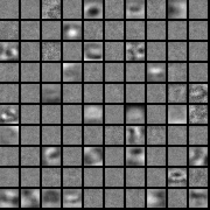
Quite a large portion of the weights are nearly zerod out. The remaining ones have managed to learn a general contrast pattern. It’s interesting to see how smooth they are. I wonder if there is an implicit L2 weight decay, like we saw in the previous post, from introducing the sparsity penalty. There are also some patterns that look like they’re still forming but not quite finished.

The results are certainly encouraging but there might be an efficiency drawback. Seeing as a lot of the weights are zeroed out, it means we have to use more hidden units in the hope of finding more meaningful patterns. If I keep the same number of units but increase the sparsity target then it approaches the random like patterns.

Download

RBM_Features-0.1.0.tar.gz

Have a look at the README.txt for instructions on obtaining the CIFAR dataset.

RBM, L1 vs L2 weight decay penalty for images

Last Updated on February 13, 2013 by nghiaho12

I’ve been fascinated for the past months or so on using RBM (restricted Boltzmann machine) to automatically learn visual features, as oppose to hand crafting them. Alex Krizhevsky’s master thesis, Learning Multiple Layers of Features from Tiny Images, is a good source on this topic. I’ve been attempting to replicate the results on a much smaller set of data with mix results. However, as a by product of I did manage generate some interesting results.

One of the tunable parameters of an RBM (neural network as well) is a weight decay penalty. This regularisation penalises large weight coefficients to avoid over-fitting (used conjunction with a validation set). Two commonly used penalties are L1 and L2, expressed as follows:

weight\;decay\;L1 = \displaystyle\sum\limits_{i}\left|\theta_i\right|

weight\;decay\;L2 = \displaystyle\sum\limits_{i}\theta_i^2

where theta is the coefficents of the weight matrix.

L1 penalises the absolute value and L2 the squared value. L1 will generally push a lot of the weights to be exactly zero while allowing some to grow large. L2 on the other hand tends to drive all the weights to smaller values.

Experiment

To see the effect of the two penalties I’ll be using a single RBM with the following configuration:

  • 5000 input images, normalized to \mu=0, \sigma=1
  • no. of visible units (linear) = 64 (16×16 greyscale images from the CIFAR the database)
  • no. of hidden units (sigmoid) = 100
  • batch training size = 100
  • iterations = 1000
  • momentum = 0.9
  • learning rate = 0.01
  • weight refinement using an autoencoder with 500 iterations and learning rate of 0.01

The weight refinement step uses a 64-100-64 autoencoder with standard backpropagation.

Results

For reference, here are the 100 hidden layer patterns without any weight decay applied:

As you can see they’re pretty random and meaningless There’s no obvious structure. Though what is amazing is that even with such random patterns you can reconstruct the original 5000 input images quite well using a weighted linear combinations of them.

Now applying an L1 weight decay with a weight decay multiplier of 0.01 (which gets multiplied with the learning rate) we get something more interesting:

We get stronger localised “spot” like features.

And lastly, applying L2 weight decay with a multiplier of 0.1 we get

which again looks like a bunch of random patterns except smoother. This has the effect of smoothing the reconstruction image.

Despite some interesting looking patterns I haven’t really observed the edge or Gabor like patterns reported in the literature. Maybe my training data is too small? Need to spend some more time …

HP Pavilion DM1 + AMD E-450 APU, you both suck!

Last Updated on February 6, 2013 by nghiaho12

Last year I bought myself a small HP Pavilion DM1 for traveling overseas. On paper the specs look great compared to any of Asus EEE PC offering in terms of processing power and consumption. It’s got a dual core AMD E-450, Radeon graphics card,  2GB RAM and about 4-5 hrs of battery life. In reality? I’ve had to take this laptop in for warranty repair TWICE in a few short months. First time was a busted graphics chip that only worked if I plugged in an external monitor. The second time was a faulty hard disk singing the click of the death. Both were repaired within a day, so I can’t get too mad. But when I finally got around to installing all the tools I need to do some number crunching under Linux, this happens …

Yes that’s right, Octave crashes on a matrix multiply!!! WTF?!?

I ran another program I wrote in GDB and it reveals this interesting snippet

My guess is it’s trying to call some AMD assembly instruction that doesn’t exist on this CPU. Octave uses /usr/lib/libblas as well, which explains the crash earlier. Oh well, bug report time …