Last Updated on January 6, 2012 by nghiaho12
I came across this topic while searching for a fast Gaussian implementation. It’s approximating a Gaussian by using multiple box filters. It’s old stuff but cool nonetheless. I couldn’t find a reference showing it in action visually that I liked so I decided to whip one up quickly.
The idea is pretty simple, blur the image multiple times using a box filter and it will approximate a Gaussian blur. The box filter convolution mask in 1D looks something like [1 1 1 1] * 0.25 , depending how large you want the blurring mask to be. Basically it just calculates the average value inside the mask.
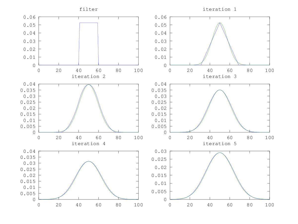
Alright enough yip yapping, lets see it in action! Below shows 6 graphs. The first one labelled ‘filter’ is the box filter used. It is a box 19 units wide, with height 1/19. Subsequent graphs are the result of recursively convolving the box filter with itself. The blue graph is the result of the convolution, while the green is the best Gaussian fit for the data.

After the 1st iteration the plot starts to look like a Gaussian very quickly. This link from Wikipedia says 3 iterations will approximate a Gaussian to within roughly 3%. It also gives a nice rule of thumb for calculating the length of the box based on the desired standard deviation.
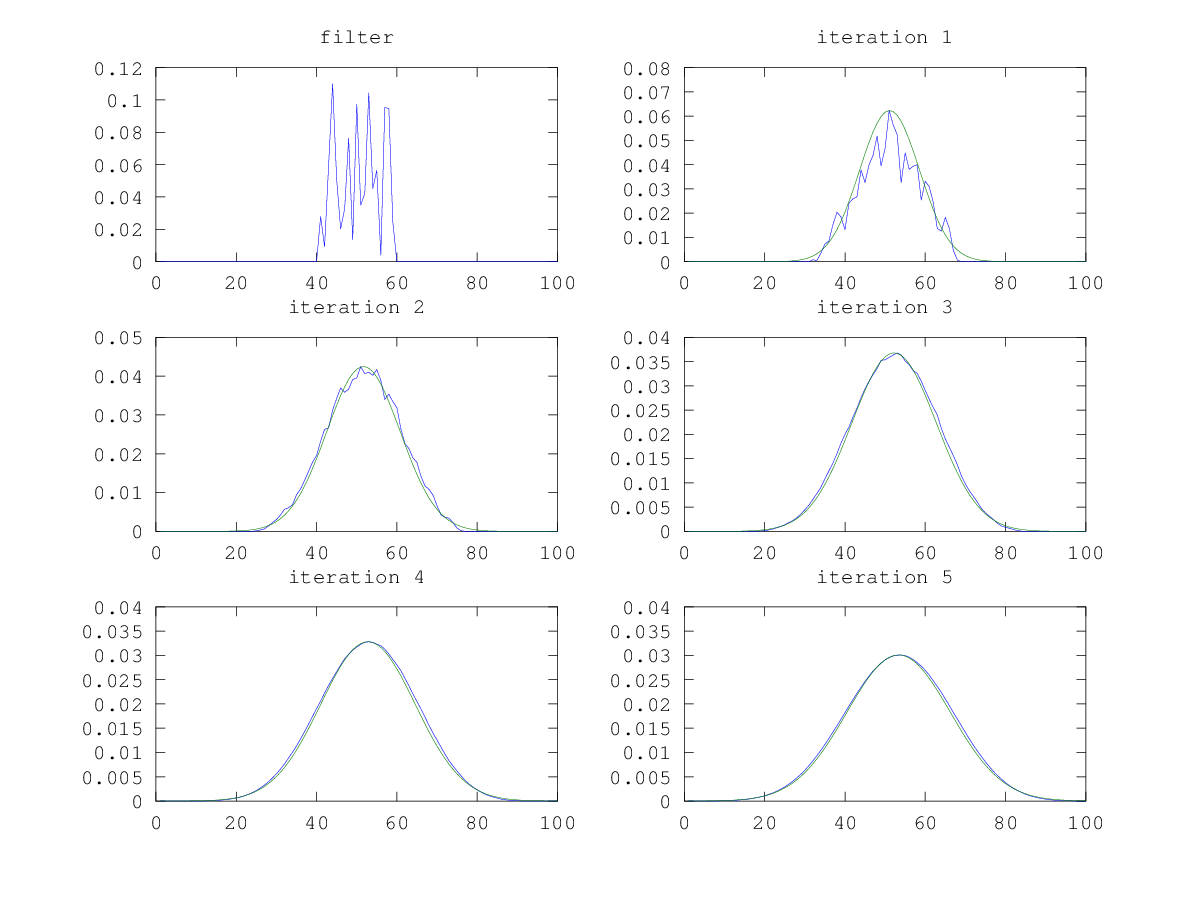
What’s even cooler is that this works with ANY filter, provided all the values are positive! The graph below shows convolving with a filter made up of random positive values.

The graph starts to smooth out after the 3rd iteration.
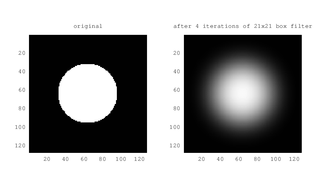
Another example, but with an image instead of a 1D signal.
 For the theory behind why this all works have a search for the Central Limit Theorem. The Wikipedia article is a horrible read if you’re not a maths geek. Instead, I recommend watching this Khan Academy video instead to get a good idea.
The advantage of the box filter is that it can be implemented very efficiently for 2D blurring by first separating the mask into 1D horizontal/vertical mask and re-using calculated values. This post on Stackoverflow has a good discussion on the topic.
Code
You can download my Octave script to replicate the results above or fiddle around with. Download by right clicking and saving the file.
Hi,
Thanks for your article.
I want say to you that the same theory was explained in a report from Peter Kovesi
And a code framework is also available
http://www.csse.uwa.edu.au/~pk/research/matlabfns/#integral
Tech report describing high speed approximate Gaussian filtering via integral images.
=>http://web.csse.uwa.edu.au/research/?a=826172
I have test it in C++, but it is not so fast….
Regards,
Pierre M
Ah I remember that page! I knew I saw it somewhere before … The fastest Gaussian Blur I’ve seen so far is in OpenCV. Unfortunately, their code is buried in layers and layers of code, which makes it hard to go through. On my lalptop OpenCV 2.3 does a Gaussian blur with sigma = 1.6 on a 640×480 greyscale image in like 2-3 ms.
really nice post. Don’t know is there any comparision result of different Gaussion filter approach.
Not that I know of.
Hello sir. I am using 2D gaussian in matlab by the code:
Ksigma=fspecial(‘gaussian’,round(2*sigma)*2 + 1,sigma);
OK. Now I want to use your code. Hence, It is converted to:
sigma=5; Ksigma = ones(2*sigma+1,2*sigma+1);
Ksigma = Ksigma/sum(Ksigma(:));
Is it correct? But I did not see any advantage of box filter. Can you suggest to me some its advantage when I use it for convolution? For example KI = imfilter(Img,Ksigma,’replicate’); %Img is image
Your code looks correct. Honestly, I don’t think there’s any advantage in using a box filter in practice.
Thank you. Your box is defined by mathematic as
f(||u||)=1 for ||u||≤σ and 0 elsewhere
Is it right? Do you have any paper about your kernel. I want to cite it in my paper. BTW, your paper looks average kernel.
To avoid confusing mathematics, if my kernel is width of 7, then all the values inside are 1/7. So it just averages all the pixels inside the kernel. I used Wikipedia. So you can find papers cited there,
Nice article. Yes, it will work with any filter, as long as it is not too mean.
The reason box filters are usually used though, is that the resulting convolution can be calculated very quickly by first calculating the primitive function F(x), which is done iteratively with the formula F(x) = F(x-1) + f(x), and then calculating the convolution as F(x+r) – F(x-r-1), where r is the “radius” of the box filter (so the box filter covers 2*r+1 values).
The method will also approximate a Gaussian even better if you vary the size of the box filter in each iteration. So the sizes of the box filters if you have three of them may be for example 8 pixels, 10 pixels and 12 pixels respectively, instead of just being 10 pixels for all filters.