Last Updated on July 7, 2013 by nghiaho12
This is a continuation from the last post. This time I implemented translation + horizontal flipping. The translation works by cropping the 32×32 image into smaller 24×24 sub-images (9 to be exact) to expand the training set and avoid over fitting.
This is the network I used
- Layer 1 – 5×5 Rectified Linear Unit, 64 output maps
- Layer 2 – 2×2 Max-pool
- Layer 3 – 5×5 Rectified Linear Unit, 64 output maps
- Layer 4 – 2×2 Max-pool
- Layer 5 – 3×3 Rectified Linear Unit, 64 output maps
- Layer 6 – Fully connected Rectified Linear Unit, 64 output neurons
- Layer 7 – Fully connected linear units, 10 output neurons
- Layer 8 – Softmax
Below is the validation error during training. I’ve changed the way the training data is loaded to save memory. Each dataset is loaded and trained one at a time, instead of loading it all into memory. After a dataset is trained I output the validation error to file. Since I use 4 datasets for training each data point on the graph represents 1/4 of an epoch (one pass through all the training data).
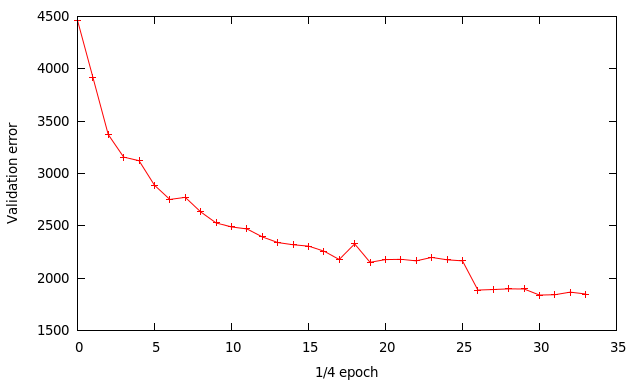
I used an initial learning rate of 0.01, then changed to 0.001 at x=26 then finally 0.0001 at x=30. The other training parameters are
- momentum = 0.9
- mini batch size = 64
- all the data centred (mean subtracted) prior to training
- all weights initialised using a Gaussian of u=0 and stdev=0.1 (for some reason it doesn’t work with 0.01 like most people do)
The final results are:
- training error ~ 17.3%
- validation error ~ 18.5%
- testing error ~ 20.1%
My last testing error was 24.4% so there is some slight improvement, though at the cost of much more computation. The classification code has been modified to better suit the 24×24 cropped sub-images. Rather than classify using only the centre sub-image all 9 sub-images are used. The softmax results from each sub-image is accumulated and the highest score picked. This works much better than using the centre image only. This is idea is borrowed from cuda-convnet.
Here are the features learnt for the first layer.
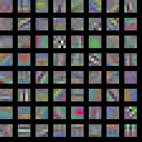
Using cropped sub-images and horizontal flipping the training set has expanded 18 times. The error gap between training error and validation error is now much smaller than before. This suggests I can gain improvements by using a neural network with a larger modeling capacity. This is true for the network used by cuda-convnet to get < 13% training error. Their network is more complex than what I’m using to achieve those results. This seems to be a ‘thing’ with neural networks where to get that extra bit of oomph the complexity of the network can grow monstrously, which is rather off putting.
Based on results collected for the CIFAR-10 dataset by this blog post the current best is using something called a Multi-Column Deep Neural Network, which achieves an error of 11.21%. It uses 8 different convolution neural networks (dubbed ‘column’) and aggregate the results together (like a random forest?). Each column receives the original RGB images plus some pre-processed variations. The individual neural network column themselves are fairly big beasts consisting of 10 layers.
I think there should be a new metric (or maybe there already is) along the lines of “best bangs for bucks”, where the state of the art algorithms are ranked based on something like [accuracy]/[number of model parameters], which is of particular interest in resource limited applications.
Download
To compile and run this code you’ll need
- CodeBlocks
- OpenCV 2.x
- CUDA SDK
- C++ compiler that supports the newer C++11 stuff, like GCC
Instructions are in the README.txt file.
Dear Nghia Ho,
Please, could you tell me the steps how to compile the code using CodeBlocks ?
Best
Hayder
There’s not much to it. Get codeblocks and load the project and hit compile.
Thank you so much. The code succeffully run but it sticks with validation error =8986. I chose the learning rate 0.01 then I changed it to 0.001 as you did but I got the same result.
Yeah it’s a black art. Took me a while to get to those errors.
So please, how can fix them ? OR could I have the the right one ? I am really appreciate you
Honestly, I have no idea. I haven’t touched this for a long time 🙂
Hi nghiaho,
Thanks for sharing these, I have some questions about your cnn.
I can’t quite understand your network structure, you use “64 output maps” in each conv layer, so after 3 layers of convolution, there are 64*64*64=262,144 outputs, and all of them are 3-channel, right? Then how could you use 64 neurons in the full-connected layer to deal with so many inputs? Is there anything I misunderstood? Thank you.
Hi,
Thanks for your enquiry, it actually helped me jog my memory of how I even wrote this complex beast. So for the first layer this is how it works
Input is 32×32 RGB, split into 3 channels
For each channel apply 64 ‘5×5 Rectified Linear Unit filters’
If you merge the RGB output from the Recitifed Linear units you get the pretty filters. So there are a total of 64 + 64 + 64 filters.
Thanks for replying.
Yeah what you’re saying is 1st conv-layer, right? We can see it as 64 filters and each of which has 3 channels (RGB, YCrCb or whatever). Then what about the 2nd layer? Say we have only one input image (3-channel), and convolved with 1st layer, we actually get 64 3-channel images (kernel size of 1st layer is 5*5, so these output images are 28*28, and after pooling, 14*14 images). If your 2nd layer is still 64 kernels, then the output of 2nd conv-layer should be 64*64, right?
Yep, what I described is for layer 1. After pooling from layer 2 you get the 14×14 images as you described. The process then repeats itself for layers 3 and 4. For each RGB channel I take the 14×14 images, convolve it with a new set of 64 5×5 filters, which results in 8×8 images. In layer 4, pooling then reduces it down to 4×4.
It gets pretty confusing I know, it took me a while too 😉