Last Updated on January 8, 2012 by nghiaho12

This post on how to take advantage of the Harris corner to calculate dominant orientations for a feature patch, thus achieving rotation invariance. Some popular examples are the SIFT/SURF descriptors. I’ll present an alternative way that is simple to implement, especially if you’re already using Harris corners.

Background

The Harris corner detector is an old school feature detector that is still used today. Given an NxN pixel patch, and the horizontal/vertical derivatives extracted from it (via Sobel for example), it accumulates the following matrix

$A = \frac{1}{N^2} \left[\begin{array}{cc} I_{x}^2 & I_{x}I_{y} \\ I_{x}I_{y} & I_{y}^2 \end{array} \right]$

where

$I_{x}$ is the summation of the derivatives in the x direction and $I_{y}$ in the y direction for every pixel. The $\frac{1}{N^2}$ averages the summation. Mathematically you don’t really need to do this, but in practice due to numerical overflow you want to keep the values in the matrix reasonably small. The 2×2 matrix above is the result of doing the following operation

Let $B = \left[\begin{array}{cc} ix_{1} & iy_{1} \\ ix_{2} & iy_{2} \\ . & . \\ . & . \\ ix_{n} & iy_{n} \end{array} \right]$

where $ix_{n}$ and $iy_{n}$ are the derivatives at pixel n.

Using B we get

$A = B^{T}B$

You can think of matrix A as the covariance matrix, and the values in B are assumed to be centred around zero.

Once the matrix A is calculated there are a handful of ways to calculate the corner response of the patch, which I won’t be discussing here.

Rotation invariance

With the matrix A, the orientation of the patch can be calculated using the fact that the eigenvectors of A can be directly converted to a rotation angle as follows (note: matrix are index as A(row,col) )

$t = trace(A) = A(1,1) + A(2,2)$

$d = determinant(A) = A(1,1)*A(2,2) - A(1,2)*A(2,1)$

$eig1 = t/2 + \sqrt{t^{2}/4 - d}$

$angle = atan2\left(A(2,1), eig1 - A(2,2)\right)$

eig1 is the larger of the two eigenvalues, which corresponds to the eigenvector

$v = \left[\begin{array}{c} eig1 - d \\ A(2,1) \end{array} \right]$

The eigenvalue/eigenvector was calculated using an algebraic formula I found here.

I’ve found in practice that the above equation results in an uncertainty in the angle, giving two possibilities

angle1 = angle

angle2 = angle + 180 degrees

I believe this is because an eigenvector can point in two directions, both of which are correct. If v is an eigenvector then -v is legit as well. A negation means a 180 degree rotation. So there are in fact two dominant orientations for the patch. So how do we resolve this? We don’t, keep them both!

Example

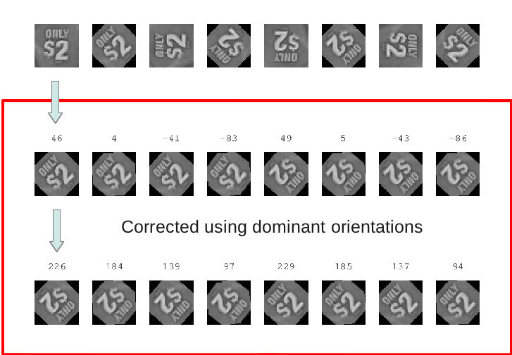
Here’s an example of a small 64×64 patch rotated from 0 to 360, every 45 degrees. The top row is the rotated patch, the second row is the rotation corrected patch using angle1 and the third row using angle2. The numbers at the top of the second/third rows are the angles in degrees of the rotated patches. You can see there are in fact only two possible appearances for the patch after it has been rotated using the dominant orientation.

Interestingly, the orientation angles seem to have a small error. For example, compare patch 1 and patch 5 (counting from the left). Patch 1 and patch 5 differ by 180 degrees, yet the orientations are 46 and 49 degrees respectively, a 3 degree difference. I think this might be due to the bilinear interpolation when I was using the imrotate function in Octave. I’ve tried using an odd size patch eg. 63×63, thinking it might be a centring issue when rotating but still the same results. For now it’s not such a big deal.

Implementation notes

I used a standard 3×3 Sobel filter to get the pixel derivatives. When accumulating the A matrix, I only use pixels within the largest circle (radius 32) enclosed by the 64×64 patch, instead of all pixels. This makes the orientation more accurate, since the corners sometime appear off the image when they are rotated.

Code

Here is the Octave script and image patch used to generate the image above (minus the annotation). Right click and save as to download.

rotation_invariance.m

patch.png

Last Updated on January 6, 2012 by nghiaho12

I came across this topic while searching for a fast Gaussian implementation. It’s approximating a Gaussian by using multiple box filters. It’s old stuff but cool nonetheless. I couldn’t find a reference showing it in action visually that I liked so I decided to whip one up quickly.

The idea is pretty simple, blur the image multiple times using a box filter and it will approximate a Gaussian blur. The box filter convolution mask in 1D looks something like [1 1 1 1] * 0.25 , depending how large you want the blurring mask to be. Basically it just calculates the average value inside the mask.

Alright enough yip yapping, lets see it in action! Below shows 6 graphs. The first one labelled ‘filter’ is the box filter used. It is a box 19 units wide, with height 1/19. Subsequent graphs are the result of recursively convolving the box filter with itself. The blue graph is the result of the convolution, while the green is the best Gaussian fit for the data.

After the 1st iteration the plot starts to look like a Gaussian very quickly. This link from Wikipedia says 3 iterations will approximate a Gaussian to within roughly 3%. It also gives a nice rule of thumb for calculating the length of the box based on the desired standard deviation.

What’s even cooler is that this works with ANY filter, provided all the values are positive! The graph below shows convolving with a filter made up of random positive values.

Gaussian approximation using a random filter

The graph starts to smooth out after the 3rd iteration.

Another example, but with an image instead of a 1D signal.

For the theory behind why this all works have a search for the Central Limit Theorem. The Wikipedia article is a horrible read if you’re not a maths geek. Instead, I recommend watching this Khan Academy video instead to get a good idea.

The advantage of the box filter is that it can be implemented very efficiently for 2D blurring by first separating the mask into 1D horizontal/vertical mask and re-using calculated values. This post on Stackoverflow has a good discussion on the topic.

Code

You can download my Octave script to replicate the results above or fiddle around with. Download by right clicking and saving the file.

box_demo.m
box_demo2.m

Nghia Ho

Monthly Archives: January 2012

Rotation invariance using Harris corners

Background

Rotation invariance

Example

Implementation notes

Code

Approximating a Gaussian using a box filter

Code

Where boredom, free time, and curiosity meet together