Last Updated on February 19, 2013 by nghiaho12
This is a follow up on my last post about trying to use RBM to extract meaningful visual features. I’ve been experimenting with a sparsity penalty that encourages the hidden units to rarely activate. I had a look at ‘A Practical Guide to Training Restricted Boltzmann Machines’ for some inspiration but had trouble figuring out how their derived formula fits into the training process. I also found some interesting discussions on MetaOptimize pointing to various implementations. But in the end I went for a simple approach and used the tools I learnt from the Coursera course.
The sparsity is the average probability of a unit being active, so they are applicable to sigmoid/logistic units. For my RBM this will be the hidden layer. If you look back in my previous post you can see the weights generate random visual patterns. The hidden units are active about 50% of the time, hence the random looking pattern.
What we want to do is reduce the sparsity so that the units are activated on average a small percentage of the time, which we’ll call the ‘target sparsity’. Using a typical square error, we can formulate the penalty as:
^2")
\right)")
- K is a constant multiplier to tune the gradient step.
- s is the current sparsity and is a scalar value, it is the average of all the MxN matrix elements.
- t is the target sparsity, between [0,1].
Let the forward pass starting from the visible layer to the hidden layer be:

")

- w is the weight matrix
- x is the data matrix
- b is the bias vector
- z is the input to the hidden layer
The derivative of the sparsity penalty, p, with respect to the weights, w, using the chain rule is:

The derivatives are:
 \;\; \leftarrow scalar")

")

The derivative of the sparsity penalty with respect to the bias is the same as above except the last partial derivative is replaced with:

In actual implementation I omitted the constant 
Results
I used an RBM with the following settings:
- 5000 input images, normalized to
- no. of visible units (linear) = 64 (16×16 greyscale images from the CIFAR the database)
- no. of hidden units (sigmoid) = 100
- sparsity target = 0.01 (1%)
- sparsity multiplier K = 1.0
- batch training size = 100
- iterations = 1000
- momentum = 0.9
- learning rate = 0.05
- weight refinement using an autoencoder with 500 iterations and a learning rate of 0.01

and this is what I got
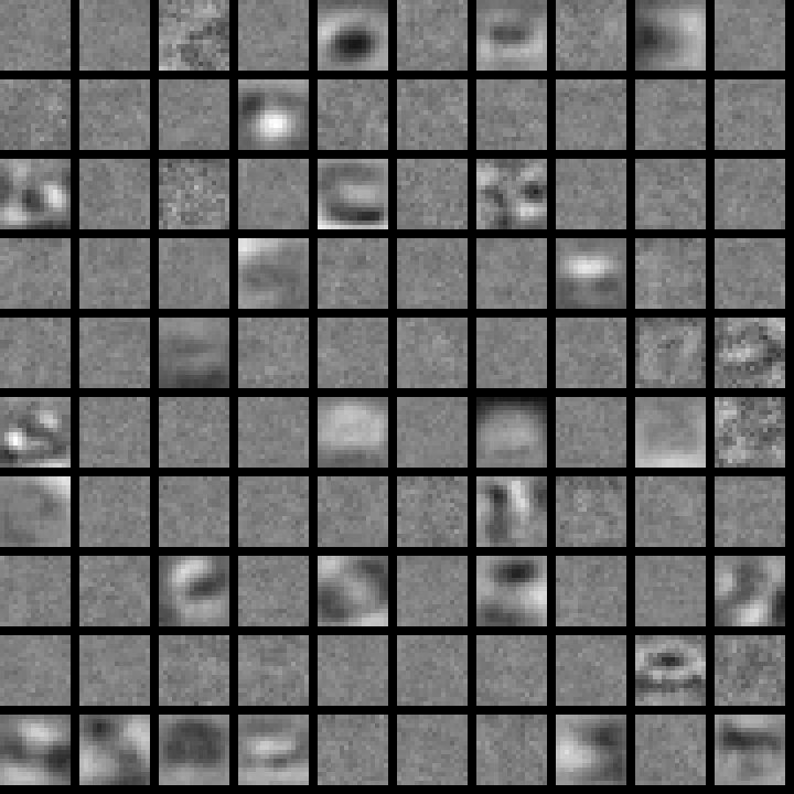 Quite a large portion of the weights are nearly zerod out. The remaining ones have managed to learn a general contrast pattern. It’s interesting to see how smooth they are. I wonder if there is an implicit L2 weight decay, like we saw in the previous post, from introducing the sparsity penalty. There are also some patterns that look like they’re still forming but not quite finished.
The results are certainly encouraging but there might be an efficiency drawback. Seeing as a lot of the weights are zeroed out, it means we have to use more hidden units in the hope of finding more meaningful patterns. If I keep the same number of units but increase the sparsity target then it approaches the random like patterns.
Download
Have a look at the README.txt for instructions on obtaining the CIFAR dataset.
Have you tried tweaking the model, perhaps using more layers? What I seem to understand from Hinton’s Coursera, and various other papers is that performance increases significantly when using multiple layers vs using just a single layer.
I was focusing on a single layer because that should be enough to get the “edge” features. My aim was to try and replicate the results from other people’s paper. Not quite there yet. I’ve put it on hold for the moment, might re-visit it when I get the chance.
Thanks for this detailed post. It helped me see how to implement a sparsity penalty for RBM learning.
However, although your derivation looks perfectly correct, I have a problem with the dh/dz term. If you use a factor h(1-h) to compute the penalty, it means that if a unit is firmly on (h=1), it will have no penalty because h(1-h) will become 0. And so it seems to me that this penalty will only act on units that are activated about 50% of the time, but it will have no effect on units that are firmly on or firmly off.
Can you help me understand how this penalty can indeed force most hidden activities to 0 (i.e. achieve sparsity)?
As for the interpretation of what is written in ‘A Practical Guide to Training Restricted Boltzmann Machines’, it is stated “For logistic units, this has a simple derivative of q-p with respect to the total input to a unit”. So I would consider that q-p is dp/dz and you would only need to multiply it by dz/dw for weights, and by dz/db for biases to obtain the penalty term. What do you think?
Hi,
You’re right that if h=1 h(1-h) will always be off but because h = sigmoid(…) it is a float between (0,1) (non-inclusive). In practice, as long as z isn’t too big h won’t be exactly 0 or 1. It can get close like h=0.99999.
Keep in mind that h(1-h) is just part of the gradient for dp/dw, not the actual penalty! It’s just used for the gradient stepping part of the optimization.
Hmm good point about the dp/dz! It sounds very logical, maybe I took a more convoluted path than I needed to. You can give it a try if you’re using my code. Go to line 92 of RBM.cpp, that’s where the sparsity stuff is done.